CHEN 1703 MIDTERM EXAMINATION Problem 1 (10 pts)

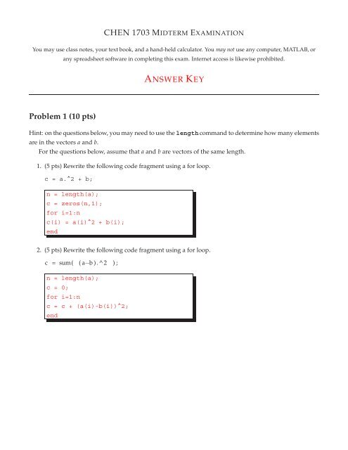
CHEN 1703 MIDTERM EXAMINATIONYou may use class notes, your text book, and a hand-held calculator. You may not use any computer, MATLAB, orany spreadsheet software in completing this exam. Internet access is likewise prohibited.ANSWER KEYProblem 1 (10 pts)Hint: on the questions below, you may need to use the length command to determine how many elementsare in the vectors a and b.For the questions below, assume that a and b are vectors of the same length.1. (5 pts) Rewrite the following code fragment using a for loop.c = a.^2 + b;n = length(a);c = zeros(n,1);for i=1:nc(i) = a(i)^2 + b(i);end2. (5 pts) Rewrite the following code fragment using a for loop.c = sum( ( a−b ) . ^ 2 ) ;n = length(a);c = 0;for i=1:nc = c + (a(i)-b(i))^2;end

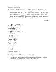
Problem 2 (10 pts)In class, and for homework 7 we discussed interpolation of vapor pressure data.following table to answer the questions belowUse the data in theT ( ◦ C) 10 20 30 40 50 60 70 80c (mm Hg) 9.21 17.5 31.8 55.3 92.5 149 234 3551. (4 pts) Estimate the vapor pressure at 51.2 ◦ C using linear interpolation. Show your work.( )p2 − pp =1(T − TT 2 − 1 ) + p 1T( 1)149 − 92.5=(51.2 − 50) + 92.560 − 50= 99.3 mm Hg.2. (6 pts) Show the system of equations that must be solved to estimate the vapor pressure at 37.5 ◦ Cusing a quadratic polynomial, p = a 0 + a 1 T + a 2 T 2 . Specifically,(a) (5 pts) Show the system of equations that must be solved to obtain the coefficients a 0 , a 1 , and a 2 .Write these in Matrix form.(b) (1 pts) Given the values for the coefficients, show how to obtain the vapor pressure at 37.5 ◦ C.⎡⎢⎣1 T 1 T 2 11 T 2 T 2 21 T 3 T 2 3⎤ ⎛⎥ ⎜⎦ ⎝⎞a 0a 1a 2⎟⎠ =⎛⎜⎝⎞p 1⎟p 2 ⎠ ,p 3substituting numbers, we have⎡ ⎤1 30 30 2⎢⎣ 1 40 40 2 ⎥⎦1 50 50 2⎛⎜⎝⎞a 0a 1a 2⎟⎠ =⎛⎜⎝31.855.392.5⎞⎟⎠ .Once we solve this for the coefficients, we obtain the pressure asp = a 0 + a 1 · 37.5 + a 2 · 37.5 2 .

Problem 3 (10 pts)For a first order reaction (like radioactive decay), the concentration as a function of time is given bywhere k is the rate constant and c 0 is the initial concentration.Use the following measurements of c(t) to answer the questions below.c = c 0 exp(−kt) , (1)t (s) 3.67e-01 9.88e-01 3.77e-02 8.85e-01c (g/cm3) 7.67e-02 6.95e-04 6.02e-01 1.15e-031. (7 pts) Determine the value for rate constant k in equation (1) that best fits the data above. Assumethat c 0 = 1.0 is known precisely. Be sure to show your work!Rearranging (1) we find( ) cln = −kt,c 0which looks like y = ax, where y ≡ ln(cc 0), a = k, and x = −t. We then have the system of equations⎛⎡ ⎤−t 1−t 2⎢⎣ −t⎥ (k) = 3 ⎦ ⎜⎝−t 4( )lnc1(c 0)lnc2(c 0)lnc3(c 0)lnc4c 0⎞⎟⎠and the normal equations are⎡[]−t 1 −t 2 −t 3 −t 4 ⎢⎣Plugging in numbers we find⎛⎤−t 1−t 2[]−t⎥ (k) = −t 1 −t 2 −t 3 −t 4 3 ⎦ ⎜⎝−t 44∑ t 2 ii=1kk == −4∑i=1( )cit i lnc 0− ∑ 4 i=1 t i ln(cic 0)∑ 4 i=1 t2 i( )lnc1(c 0)lnc2(c 0)lnc3(c 0)lnc4c 0⎞⎟⎠k= − ( 0.367 · ln ( 7.67 × 10 −2) + 0.988 · ln ( 6.95 × 10 −4) + 0.0377 · ln (0.602) + 0.885 · ln ( 1.15 × 10 −3))0.367 2 + 0.988 2 + 0.0377 2 + 0.885 2= 7.46.2. (3 pts) Determine the R 2 value (for c) as we defined it in class.

( ) 2R 2 = 1 − ∑n i=1 ci − c pred∑ n i=1 (c i − ¯c) 2 ,where c pred is the predicted value for c. First, let’s calculate¯c = 1 nNow let’s calculate the predicted compositionsusing the value for k that we obtained above.n∑ c i = 0.1701.i=1c pred = exp(−kt i ) ,[]c pred = 6.48 × 10 −2 6.31 × 10 −4 0.755 1.36 × 10 −3Now for R 2 we haveR 2 = 0.9068.