Navigation for an Intelligent Mobile Robot - IEEE Xplore

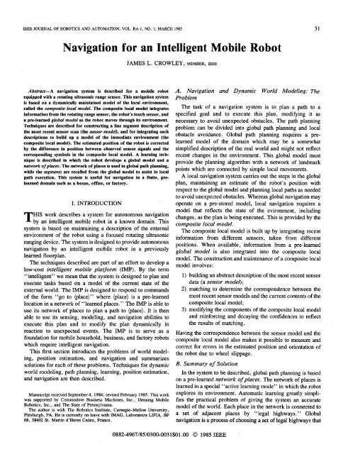
CROWLEY: NAVIGATION FOR AN INTELLIGENT ROBOT 33a sequence of points that are adjacent to the expandedobstacles. If there is position error in the control of the pathexecution, such points can possibly result in a collision.Brooks has recently proposed a new approach to the find-pathproblem based on modeling free space [2]. Brooks’ solution,developed in a two-dimensional plane, involved fitting twodimensional“generalized cylinders” to the space betweenobstacles to obtain pathways in which the object may freelytravel on a plane. The technique was extended to the thirddimension by stacking planes.B. The Stanford Cart and the C-MU RoverMoravec [8] developed a navigation system based onsensory signals using the Stanford cart. This cart sensed itsenvironment using a set of nine stereo images obtained from asliding camera. A set of candidate points were obtained in eachimage with an “interest” operator. Small local correlationswere then made at multiple resolutions to arrive at a depthestimate for the points. The matched points were plotted on atwo-dimensional grid and then expanded to a circle. A bestFig. 2. Framework for intelligent navigation system.path from the current location to a goal was then chosen as theshortest sequence of line segments which were tangent to theIII. THE COMPUTATIONAL FRAMEWORKcircles. The cart would advance by 3 ft and then repeat thesensing and planning process. Stereo matching was also A. The Composite Local Modelperformed between the images taken at different steps to The navigation system of the IMP is based on theobtain confirming and additional depth information. A new computational framework shown in Fig. 2. At the core of thisvehicle, called the C-MU Rover [9], has recently been framework is a dynamic model of the surface and obstacles inconstructed by Moravec to support these techniques. the immediate environment of the IMP called the compositelocal model. “Local” refers to the fact that only informationC. Hilarein the local environment of the IMP is represented. “Composite”refers to the fact that this model is composed ofA team under the direction of George Giralt at the LAASlaboratory in Toulouse has been investigating the design andcontrol of mobile robots since 1977. They have developed ainformation obtained over time from multiple sensors andmobile robot named Hilare. Chatila developed a navigationsystem for Hilare that is based on dividing a pre-learned floorplan into convex regions [3]. Convex regions were formed byconnecting nearest vertices to form areas called C-Cells.Laumond, at the LAAS in Toulouse, extended this idea bydeveloping hierarchies of C-Cells to represent rooms and partsof a known domain [6].D. CommentMotion Commandsfrom many views.The composite local model plays two fundamental roles inthis computational framework.1) It is the structure in which potentially conflictinginformation from diverse sensors is integrated withrecently observed information and information recalledfrom long term storage (the Global Model).2) It is the structure on which processes for local pathplanning, path execution, learning, object tracking,object recognition, and other “higher level” processesare based.A few other efforts towards developing autonomous mobile Because of the nature of the navigation task and the sensorsrobots have also been reported. In many cases the efforts focus that are employed, the composite local model in the IMP ison engineering problems and pay little attention to the issues of implemented with a relatively simple 2-D representation. Theworld modeling or path planning [lo]. Other groups have IMP models the world and plans paths in a 2-D “flat-land’’become bogged down on the vision problem, often spending universe. Because the rotating range sensor is mounted at atheir efforts on general solutions to the problems of low level height of 30 in, the robot is able to detect and represent most ofvision. We believe that the most important problems to be the furniture that it encounters. Surfacesandobstacles areaddressed now are sensor interpretation, navigation, andsystem organization. Toward this end, we have developed arepresented as connected sequences of line segments. Thus atable and a wall have the same structure; both appear as acomputational paradigm for intelligent robotic systems. Thiscomputational paradigm provides a framework for the procbarrierwith andimension.infinite (or unknown) extent in verticalesses involved in sensor interpretation, path planning, and The composite local model must include the ability topath execution.represent the uncertainty of information. In this system,

34 IEEE JOURNAL OF ROBOTICS AND AUTOMATION, VOL. RA-1, NO. 1, MARCH 1985confidence is represented by a set of states. The line segmentswhich compose the composite local model include a “state”attribute which represents the degree of confidence. Consistentline segments are reinforced and extended while inconsistentline segments are decayed and eventually removed fromthe model. Representing uncertainty with states permits easyimplementation of arbitrary rules for reinforcement and decay.B. The Sensor ModelsSensors typically produce large amounts of information.Before the information from a sensor can be integrated into thecomposite local model, surface information must be abstractedfrom it. The sensor model may be viewed as a form of logicalsensor which provides the sensor information in a standardform which may be integrated into the composite localmodel.In the first version of the IMP, the sensors are a set ofcontact sensors on a skirt and the rotating sonar sensor. In eachcase, the sensor model is an abstract description expressed asline segments which represent surfaces in the real world.C. Match and UpdateThe module labeled “match” determines the correspondencebetween the line segments which compose the sensormodel and the line segments which compose the compositelocal model. The correspondence is then used to determineerrors in the estimated position and to update the position,length, and confidence of the segments in the composite localmodel. Special procedures also exist for detecting and trackingmoving objects.The module labeled “update” integrates the informationfrom the sensor models with the current composite localmodel. This module adjusts the position, size, connectivity,and confidence of the segments in the composite local model toreflect the results of correspondence matching. This updateprocess also removes segments for which the confidence islow or for which the distance is too far. The process does notremove nearby surfaces which are not currently visible.IV. CONSTRUCTING AN ABSTRACT DESCIUPTIQNOF RANGE DATADepth readings from the rotating sonar are converted intoline segments by a sequence of four steps.Project the reading to a Cartesian world coordinatesystem.Segment measured points into line segments by detecting“discontinuities” and then applying a recursive linefitting process.Compute the line equations of the points from the mostreliable interior points.Recompute the segment endpoints as the intersectionpoints with neighboring line segments.These processes are described below.A. Projection to Cartesian World CoordinatesDepth readings are obtained from the rotating sonar incylindrical coordinates, i.e., as depth at a particular angle. Aseach depth reading is made, the current estimated position andorientation of the IMP is affixed to it. This permits the system0 RobotFig. 3. Edges of sonar beam are projectedSonar BeamsSurf aceto world coordinates.to project the reading into a world coordinate system at a latertime, even if the data were taken while the IMP was moving.As a consequence of the detection mechanism in the sonar,the depth reading refers to the depth to the nearest reflectingsurface anywhere in the sonar beam’s circular footprint. Whenthe beam reflects from a flat surface at a non-perpendicularangle, the sonar returns the distance along the short edge of thebeam. Knowledge of this physical process is used in interpretingthe sonar depth readings.As each sonar reading is obtained, it is converted fromrobot-centered polar coordinates to a world-centered Cartesiancoordinate system. This is done by projecting a line by thespecified depth at the specified angle, as illustrated in Fig. 3. Ifthe readings are decreasing as the sonar rotates in a counterclockwiseturn, the angle is adjusted to be the left edge of thebeam by adding the estimated half angle of the sonar beam. Ifthe depth is increasing, the angle is adjusted to the right bysubtracting the estimated half angle. The difference in depthbetween the adjacent readings to the right and to the left iscomputed and affixedmeasure.to the projected beam as a qualityB. Segmenting the Points Into Line SegmentsThe points are first grouped into a sequence of roughly colinearreadings such that the distance between each adjacentpair of points is less than a tolerance. This tolerance is selectedas a compromise between the maximum distance at which thedepth readings can be taken and the smallest gap betweenobjects that the system can detect. For a difference inorientation of a degrees per reading, the minimum distancegap size Gmin is determined by the desired maximum range Rby considering the difference of beam edges for a perpendicularsurface. Such a geometry gives the relationshipG ~ > R n Tan@)In our system, cy = 3” and R = 25.6 ft, giving Gmin of 1.34ft. We have found a value of Gmin of 1.5 ft to be satisfactory.Thus, the points are scanned to detect any points where thedistance between adjacent readings is greater than 6~n. Suchpoints are called break points or discontinuity points. Breakpoints mark the boundaries of collections of points that arepassed to a recursive line fitting procedure.Recursive line fitting has been used for years to fit lines toedge points in images [5]. The algorithm is illustrated in Fig.4. A line equation of the formAx+By+C=Ois computed between the two endpoints inthe collection of

CROWLEY: NAVIGATION FOR AN INTELLIGENT ROBOT 37The correspondence types are used to extend thecomposite local model segment during the update process.4) Is the segment LM the longest found so far?The correspondence function provides both the index of thecorresponding segment and the type of correspondence.D. The Update Process-- Local Model SegmentSensor Model SegmentThe update process is the mechanism by which linesegments from the sensor model, global model, and contact Fig. 7. Orientation error given by average difference in angle betweensensor enter and refine the composite local model. During sensor model segments and corresponding local model segments.each sonar scan, segments from the sensor model are matchedto the current composite local model, and the result of F. Updating the Vertex Positions and Segment StatesThe main functions of the update process are as follows.1) Increase the confidence state of transient segments forwhich there is a corresponding segment in the sensormodel.2) Decay the confidence of segments that should be visible,but for which there is not a corresponding segment the inmost recent sensor model.3) Add newly observed sensor model segments and segmentsrecalled from the global model to the compositelocal model.4) Refine the vertex position of segments which are“reinforced” by the sensor model.E. Marking the Visible Segments in the Composite LocalModelSegments in the composite local model for which there is nocorrespondence are only modified under two conditions.The segment was marked as visible during constructionof the sonar model.The nearest point on the line segment is more than a givendistance from the IMP’s current position.The second condition is a simple mechanism by whichsegments “fall off the end of the world” as the IMP movesaway from them. The actual distance is relatively unimportantas long as it is beyond the sonar range and the current area oflocal navigation. Of course, the larger this distance, the more“extra” segments the system has to consider on eachcalculation.The first condition establishes a “visible horizon” for theIMP. As each point is added to the Sensor Model, the functionVISIBLE is called, for a point at the direction of the beam and therange of the sonar, to determine which segment in thecomposite local model should be visible. If a segment is found,the difference in angle between the beam and that segment iscomputed. If this difference in angle is not small ( c 15 ”) thenthat composite local model segment is marked as visible.Segments for which the angle of incidence of the sonar beam isvery small are not detected reliably by the sonar and are thusnot marked as visible.Unconnected vertices should be extended when there is acorrespondence of types 1, 2, or 3.The position of connected vertices has precedence overthe position of an unconnected vertex.A segment is more stable when both its vertices areconnected.The actual rules for state updates are implemented as casestatements based on the current state and then ’on thecorrespondence type.After the vertex positions and states of the segments in thecomposite local model have been updated, segments from thesensor model for which there was no correspondence in thecomposite local model are added to the composite local modelin the lowest confidence state (state 1). A relabeling process isthen used to connect adjacent segments for which the verticesare very close.VI. CORRECTING THE ESTIMATED POSITIONLocal path execution and learning and updating the compositelocal model all depend critically on maintaining an accurateestimate of the IMP’s current position. An instantaneousestimate of the IMP’s position is maintained from the rotaryposition encoders on the IMP’s wheels. This estimatedposition is monitored and corrected by a process based oncomparing the sensor model to the composite local model.Before the composite local model is updated from the sensormodel, the correspondence between the sensor model and thecomposite local model is used to detect and correct anysystematic error in the estimated position of the IMP.As each sensor model line segment is obtained, thecorrespondence is found to the most likely line segment in thecomposite local model. The difference in angle between thesesegments is then computed. When a sensor model has beenconstructed from a complete scan of the rotating depth sensor,the average error in angle is computed. This average error iscomputed from the difference in orientation between SensorModel segments and the corresponding composite local modelsegments, as illustrated by Fig. 7. The sensor model is thenrotated around the position of the IMP by this average error in

38 IEEE JOURNAL OF ROBOTICS AND AUTOMATION, VOL. RA-1, NO. 1, MARCH 1985- Local Model Segment-;1.1\Sensor Model SegmentFig. 8. Position error given by average difference in position betweenconnected vertices in sensor model and corresponding connected verticesin the local model.angle, as illustrated by Fig. 8, and the average error issubtracted from the estimated orientation.Next, the average error in position is computed bycomputing the average x and y errors between connectedvertices in the rotated sensor modeland the correspondingvertices in the composite local model. This average error inposition is then subtracted from the estimated positionandfrom the position of the line segments in the sensor model. Thesegments in the composite local model are then updated toinclude the results of matching to the sensor model.VU. GLOBAL PATH PLANNING AND NAVIGATIONGlobal path planning is based on the network of places,whereas local path planning and execution are based on theinformationin the composite local model. The global pathplanning process uses the network of places to determine theshortest sequence of straight line paths that will take the IMPto a specified goal point. Global paths are planned based on anetwork of “Adit” points which are connected by straight linepaths. The path is then executed as a sequence of straight linemovements.A. Navigation ModesThere are three modes in which the IMP may travel.Learn Mode: Limited exploratory movements in an unfamiliarenvironment, with the purpose of learning the environment.Manual Mode: User specified motion executed by localnavigation.Automatic Mode: Autonomous movement to a namedgoal point in response to a command of the form “go to(place)’’.Learn mode permits the IMP to learn the global model fromwhich it constructs the network of places. Automatic mode isdesigned to permit the IMP to execute navigation tasks in thelearned environment. Manual mode is default a mode in whichthe IMP may travel to a visible point using only local straightline navigation.B. The Network of Places and the Global ModelThe learned domain of the IMP is represented in two relateddata structures: the “global model” and the “network ofplaces.” The global model is the collection of line segmentsobserved by the composite local model while making a tour ofiniFig. 9. Global model produced for typical floor plan used in simulator.tiIFig. 10. Network of placescomposed of aditsandlegalhighways.Aditsshown as boxes.the house in learn mode. The global model permits the IMP torecall the surfaces that it should observe at any location in theknown world. An example of a global model constructed bythe automatic learning processrunningon the simulator isshown in Fig. 9. The network of places is the structure whichserves as a basis for global path planning. The network ofplaces is obtained by dividing the free space in the globalmodel into convex regions. A convex region has the propertythat any two points within the region may be connected by astraight line that remains entirely within the region. Thus amobile robot may travel between any two points within aconvex region by a single straight line motion. An example ofthe convex regions for the global model shown in Fig. 9 isshown in Fig. 10.Convex regions are constructed with an algorithm which isdesigned to maximize the area of the largest convex region [4].A pair of navigation landmarks, called “adits” (an adit is theopposite of an exit), are created for each cut that is made topartition free space to create the convex regions. The adits aredisplaced to the sides of the cut so that the robot will passthrough the cut at a roughly perpendicular angle. This protectsthe robot from grazing the edges of door ways and tightspaces.Convex regions are shrunk by the diameter of the robot to

CROWLEY: NAVIGATION FOR AN INTELLIGENT ROBOT 39represent the free space in which the robot may travel. Thespace inside a doorway after shrinking forms a special regioncalled a “doorway region.” Doorway regions are not guaranteedto be convex. Each adit is connected to the adit on theother side of the doorway and to all other adits within itsconvex region, as shown in Fig. 10. In this figure, the adits tothe convex regions are illustrated with boxes.The network of places is a three level structure. At the toplevel are a list of user-defined “named places.” At the middleis a list of convex regions. Each named place points to aconvex region, and each convex region contains a list ofnamed places. Each convex region also contains a list of adits.The adits serve as landmarks to global path planning andexecution. The convex regions serve as “legal highways” forplanning paths to any named place.C. Global Path PlanningA global path is planned as a sequence of adits which willtake the robot from its current convex region to the convexregion which contains a specified goal point. A command ofthe form “go to (place)” provides a pointer to a convex regionthat in turn provides a list of possible goal adits. The aditclosest to the named place is chosen as a goal for pathplanning. Knowledge of the current convex region gives a listof adits from which to start the path. The nearest adit isselected as a starting adit. The shortest path through thenetwork of adits is determined using a version of Dijkstra’salgorithm [ 11 which halts when a path to the desired goal placehas been found. If the start (or the end) of this path leadsthrough two adits in the same region, the first (or last) adit isdropped from the path. Global path execution is then reducedto a three step process in which the IMP 1) moves to the firstadit in the path, 2) moves from each adit on the path to thenext, and 3) then moves from the last adit to the goal place.VIII. .LOCAL NAVIGATIONFig. 11. State transition diagram for local navigation.IMPFig. 12. Legal highway for pathGoalexecution.In the TURN state, the IMP turns toward the goal point untilthe difference between the estimated orientation and thedirection to the goal point falls below the minimum turningresolution. The IMP then enters the WAIT state to make acomplete sonar scan and verify the current estimated position.The sonar scan \results in an update in the estimated positionand orientation, even if there is no change in the estimatedposition or orientation. The call to the function “Set-Estimated-Position” signals the completion of the scan andcauses a transition back to the DECIDE state. If the IMP is not atthe goal, and is turned toward the goal, control will pass fromDECIDE t0 MOVE.Upon entering the MOVE state, the IMP computes theequation of the line (the path equation) from the currentlocation to the goal point. A cyclic process is then initiated inwhich the system moves forward while performing thefollowing tests as rapidly as possible.1) Verify that the distance to the goal point is decreasing.When the distance to the goal stops decreasing, the systemreturns to HOLD to wait for the next goal. If the distance is everA local straight line path is executed by a finite state processwhich monitors the position of the robot to assure that it increasing and is larger than the goal tolerance, then theremains on the desired straight line within a tolerance. This system will go into the WAIT state to take a clean view of theprocess also monitors the local model to assure that no world.unexpected obstacle blocks the path. A recursive obstacle 2) Verify that the perpendicular distance from the currentavoidance algorithm is used to plan a path around unexpected estimated position to the path line segment is below aobstacles.A. Local Path ExecutionStraight line movement to a goal point is monitored by arelatively simple finite state process. The states of this processare the set {HOLD, DECIDE, TURN, MOVE, WAIT, BLOCKED). Thetolerance. This test is illustrated by Fig. 12. It is performed byevaluating the path equation using the current estimatedposition, yielding the perpendicular distance to the pathequation. If this distance exceeds the tolerance, then the IMPwill go to WAIT.3) Verify that there is a free path to the goal. This is donestate transition diagram for this process is shown in Fig. 11. by projecting parallel line segmentsin the composite localThe process waits in the HOLD state for a goal from the global model. If the path becomes blocked, the IMP will go intopath execution process. When a goal is received, the IMP blocked state and signal for local path planning to avoid theenters the DECIDE state. In the DECIDE state it first tests thedistance to the goal. If this distance is less than a tolerance, itreturns to HOLD. If the distance is above the tolerance, theobstacle.If the IMP is in the MOVE or TURN States and its contactsensor is triggered, it immediately halts and enters the BLOCKEDdifference in angle between the current heading and the goal is state. Entering BLOCKED triggers the local path planningtested. If this angle is above the minimum resolution for procedures to plan a path around an obstacle. A lowturning,the IMP enters the TURN state; otherwise it enters theMOVE Sbb.confidence line segment is also placed into the composite localmodel to represent the obstacle.

40 IEEE JOURNAL AND AUTOMATION, OF ROBOTICSVOL. RA-I, NO. 1, MARCH 1985B. Local Obstacle AvoidanceThe purpose of local obstacle avoidance is to plan asequence of straight line paths which will take the IMP aroundan unexpected obstacle. A very simple recursive process isused, based on the segments in the composite local model.This process plans two paths, one to the left of the obstacle andone to the right. Tests are then made to see if a free path existsin the composite local model from this point to the goal andfrom this point to the current position. If either path isblocked, the procedure is called recursively to see if it ispossible to get around the blockage. The recursion is notcontinued beyond three levels.IX. LEARNING THE GLOBAL MODELThe global model is learned by a process which detects andfollows segments in the composite local model using a set ofpseudo-sensors which we have come to call “whiskers.”These pseudo-sensors are implemented in the composite localmodel using the VISIBLE function. That is, a test is made to seeif any line segments in the local model block a pair of points tothe right of the IMP at a distance of 3 ft.Learning begins by loading the current contents of theglobal model into the composite local model. The compositelocal model is then searched for the nearest potential startingpoint. A potential starting point must be a point to the left ofline segment which meets the following conditions.1) The line perpendicular to line equation and passingthrough the IMP’s position (and the starting point)intersects with the composite local model line segment.2) The function FREEPATH to the starting point from theIMP’s position must return the value true.The IMP moves directly to the nearest starting point andthen begins tracking the wall. The IMP moves in 2 foot steps,calculating each move based on the current segment. Aftereach move a sonar scan is made and then the composite localmodel is updated.There are two conditions which can cause the IMP to stoptracking the current segment. The first is where a call toFREEPATH detects a segment blocking the next goal point. Inthis case the blocking segment becomes the new currentsegment. The other condition is that where the currentsegment is no longer visible to the right. In this case the humansupervisor is asked if it is OK to turn right. If the answer isyes, the IMP proceeds in search mode, making a sequence of 1ft moves and 30” turns to the right, while searching for a newsegment to the right with its whiskers. If the answer is no, theIMP proceeds forward in moves of 2 ft, searching to the rightwith its whiskers for a new segment.Learning terminates automatically when the system comeswithin 3 ft of the first goal while tracking a segment whichcorresponds to the first segment. Learning may be terminatedby the supervisor at any time. On termination, the compositelocal model is loaded into the global model and the network ofplaces is computed by convex decomposition.An example of a learned global model and the path followedduring the learning procedure is shown in Fig. 14. The linesegments are a global model produced by the learningFig. 13. Learning global model. Left frame illustrates whiskers used indetecting presence of current segment and FREEPATH calculation used toverify next move. Boxes show ends of whiskers and next goal point.Center frame shows new segment detected by FREEPATH function. Rightframe shows IMP turning right in search of new segment to track.Fig. 14. Trace of IMP during simulated active learning. Line segmentsrepresent global model. “ + ” ’s represent actual position of IMP as ittraveled. “X” ’s represent estimated position. Errors in position ofsegments in sensor model were only source of error in experiment.”algorithm. The “ + ’s represent the actual position of theIMP as it traveled. The “X” ’s represent the estimatedposition. Errors in the position of segments produced by thesensor model were the source of error in the estimatedposition.X. SUMMARY AND CONCLUSIONThis work describes a navigation system for an intelligentmobile robot. This system is based on maintaining a dynamicmodel of the external world (the composite local model) usinga rotating depth sensor. A side effect of maintaining .thisdynamic model is an error vector which is used to maintain anestimate of the robot’s position as it moves. The dynamicallymaintained composite local model also supports the functionsof local obstacle avoidance, local planning, and learning.A path planning technique has been described that is basedon a pre-learned “network of places.” The robot’s domain isrepresented as a network of maximum-area convex regions.These convex regions serve as “legal highways” in which therobot may travel. The cuts which form these convex regionsprovide “adits” which serve as key points for planning pathsthrough the known environment. Each straight line motion isexecuted by a finite state process which monitors motion usingthe composite local model.These techniques yieldaninexpensivenavigationsystemthat is suitable for indoor environments. This system plans andexecutes paths as a sequence of straight line motions. Such

CROWLEY: NAVIGATION FOR AN INTELLIGENT ROBOTpaths are not necessarily optimal in the sense of being shortest;they are, however, a reasonable trade-off between efficiencyand safety.REFERENCESA. V. Aho, J. E. Hopcroft, and J. D. Ullman, Data Structures andAlgorithms. Reading, MA: Addison-Wesley, 1983.R. A. Brooks, “Solving the find-path problem by good representationof free space,” in Proc. Nat. Conf. Artificial Zntelligence, AAAZ-82, pp. 381-386, AUg. 1982.R. Chatila, “Path planning and environmental learning in a mobilerobot system,” in Proc. ECAZ, Orsay, France, Aug. 1982.J. L. Crowley and R. J. Redpath, “An algorithm for maximum areaconvex decomposition,” Robotics Institute, Carnegie-Mellon Univ.,Pittsburgh, PA, Tech. Rep. in preparation, 1984.R. 0. Duda and P. E. Hart, Pattern Classification and SceneAnalysis. New York: Wiley, 1973.J. P. Laumond, “Model structuring and concept recognition: Twoaspects of learning for a mobile robot,” in Proc. Eighth ZJCAZ-83,pp. 839-841, Aug. 1983.T. Lozano-Pe‘rez, “Automatic planning of manipulator transfer movements,’’ZEEE Trans. Syst., Man, Cybern., vol. SMC-11, pp. 681-698, Aug. 1981.H. P. Moravec, “Obstacle avoidance and navigation in the real worldby a seeing robot rover,” Carnegie-Mellon Robotics Institute, Pittsburgh,PA, Tech. Rep. CMU-RI-TR-3, Sept. 1980.[9] H. P. Moravec, “The CMU rover,” in Proc. Nat. Conf. ArtificialIntelligence, AAAZ-82, pp. 377-380, Aug. 1982.[lo] Y. Kanayama, “Concurrent programming of intelligent robots,” inProc. Eighth ZJCAI-83, pp. 834-838, Aug. 1983.41