4 Multiple Sequence Alignment 4.1 Multiple sequence alignment

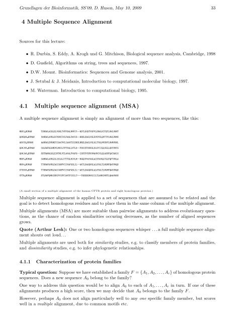
Grundlagen der Bioinformatik, SS’09, D. Huson, May 10, 2009 334 Multiple Sequence AlignmentSources for this lecture:• R. Durbin, S. Eddy, A. Krogh und G. Mitchison, Biological sequence analysis, Cambridge, 1998• D. Gusfield, Algorithms on string, trees and sequences, 1997.• D.W. Mount. Bioinformatics: Sequences and Genome analysis, 2001.• J. Setubal & J. Meidanis, Introduction to computational molecular biology, 1997.• M. Waterman. Introduction to computational biology, 1995.4.1 Multiple sequence alignment (MSA)A multiple sequence alignment is simply an alignment of more than two sequences, like this:MRP2 HUMANQ9UQ99 HUMANABCC8 HUMANQ96J65 HUMANQ96JA6 HUMANMRP5 HUMANMRP4 HUMANO75555 HUMANCFTR HUMANTSNRWLAIRLELVGNLTVFFSALMMVIY--RDTLSGDTVGFVLSNALNITQTLNWLVRMTVANRWLAVRLECVGNCIVLFAALFAVIS--RHSLSAGLVGLSVSYSLQVTTYLNWLVRMSAANRWLEVRMEYIGACVVLIAAVTSISNSLHRELSAGLVGLGLTYALMVSNYLNWMVRNLCALRWFALRMDVLMNILTFTVALLVTLS--FSSISTSSKGLSLSYIIQLSGLLQVCVRTGSSTRWMALRLEIMTNLVTLAVALFVAFG--ISSTPYSFKVMAVNIVLQLASSFQATARIGCAMRWLAVRLDLISIALITTTGLMIVLM--HGQIPPAYAGLAISYAVQLTGLFQFTVRLATTSRWFAVRLDAICAMFVIIVAFGSLIL--AKTLDAGQVGLALSYALTLMGMFQWCVRQSTTSRWFAVRLDAICAMFVIIVAFGSLIL--AKTLDAGQVGLALSYALTLMGMFQWCVRQSSTLRWFQMRIEMIFVIFFIAVTFISILT---TGEGEGRVGIILTLAMNIMSTLQWAVNSS(A small section of a multiple alignment of the human CFTR protein and eight homologous proteins.)Multiple sequence alignment is applied to a set of sequences that are assumed to be related and thegoal is to detect homologous residues and to place them in the same column of the multiple alignment.Multiple alignments (MSA) are more suitable than pairwise alignments to address evolutionary questions,as the chance of random similarities occuring decreases, as the number of aligned sequencesgrows.Quote (Arthur Lesk): One or two homologous sequences whisper . . . a full multiple sequence alignmentshouts out loud. . .Multiple alignments are used both for similarity studies, e.g. to classify members of protein families,and dissimilarity studies, e.g. to infer phylogenetic relationships.4.1.1 Characterization of protein familiesTypical question: Suppose we have established a family F = {A 1 , A 2 , . . . , A r } of homologous proteinsequences. Does a new sequence A 0 belong to the family?One way to address this question would be to align A 0 to each of A 1 , . . . , A r in turn. If one of thesealignments produces a high score, then we may decide that A 0 belongs to the family F .However, perhaps A 0 does not align particularly well to any one specific family member, but scoreswell in a multiple alignment, due to common motifs etc.

34 Grundlagen der Bioinformatik, SS’09, D. Huson, May 10, 20094.1.2 Conservation of structural elementsHere we show the alignment of N-acetylglucosamine-binding proteins to the tertiary structure of oneof them:The alignment shows exhibits 8 conserved cysteins. These form 4 disulphide bridges, which stabilizethe protein:4.1.3 MSA and evolutionary treesOne main application of multiple sequence alignments is in phylogenetic analysis. Suppose we aregiven an MSA:A ∗ 1 = N - F L SA ∗ 2 = N - F - SA ∗ 3 = N K Y L SA ∗ 4 = N - Y L SWe would like to reconstruct the evolutionary tree that gave rise to these sequences, e.g.:N Y L S N K Y L S N F S N F L S+K−LN Y L SY to FThe computation of phylogenetic trees will be discussed later.4.2 Definition of an MSASuppose we are given r sequences A i , i = 1, . . . , r over Σ:⎧A 1 = (a 11 , a 12 , . . . , a 1n1 )⎪⎨ A 2 = (a 21 , a 22 , . . . , a 2n2 )A :=.⎪⎩A r = (a r1 , a r2 , . . . , a rnr )

Grundlagen der Bioinformatik, SS’09, D. Huson, May 10, 2009 35Definition 4.2.1 (MSA) A multiple sequence alignment (MSA) of A is obtained by inserting gaps(’-’) into the original sequences such that all resulting sequences A ∗ i have equal length L ≥ max{n i |i = 1, . . . , r}, A ∗ i = A i after removal of all gaps from A ∗ i , and no column consists of gaps only.Example:A = {apple, paper, pepper}⎧⎫⎨ - a p p l e - ⎬A∗ = p a p - - e r⎩⎭p e p p - e r⎧⎪⎨A ∗ :=⎪⎩A ∗ 1 = (a ∗ 11, a ∗ 12, . . . , a ∗ 1L )A ∗ 2 = (a ∗ 21, a ∗ 22, . . . , a ∗ 2L ).A ∗ r = (a ∗ r1, a ∗ r2, . . . , a ∗ rL ),4.3 Scoring an MSAIn the case of a linear gap penalty, if we assume independence of the different columns of an MSA,then the score α(A ∗ ) of an MSA A ∗ can be defined as a sum of column scores:α(A ∗ ) :=L∑s(a ∗ 1i, a ∗ 2i, . . . , a ∗ ri).i=1Here we assume that s(a ∗ 1i , a∗ 2i , . . . , a∗ ri ) is a function that returns a score for every combination of rsymbols (including the gap symbol).For pairwise alignments there are three types of columns, a match, or a blank in either of the twosequences. The following table shows the 7 possibilities for three sequences:a 1i − a 1i a 1i − − a 1ia 2j a 2j − a 2j − a 2j −a 3k a 3k a 3k − a 3k − −For r sequences, the number of different column types iswhere i is the number of gaps.∑r−1( r= 2i)r − 1i=04.3.1 The sum-of-pairs (SP) scoreHow to define the score s? For two protein sequences, s is usually given by a BLOSUM or PAMmatrix. For more than two sequences, providing such a matrix is not practical, as the number ofpossible combinations is too large.Given an MSA A ∗ , consider two sequences A ∗ p and A ∗ q in the alignment. For two aligned symbols uand v we define:⎧⎨ match score for u and v, if u and v are residues,s(u, v) :=−dif either u or v is a gap, or⎩0 if both u and v are gaps.

36 Grundlagen der Bioinformatik, SS’09, D. Huson, May 10, 2009(Note that u = − and v = − can occur simultaneously in a multiple alignment.)The multiple alignment A ∗ induces a pairwise alignment on any two of the input sequences A p andA q .Define the score of this (not necessarily optimal) pairwise alignment ass(A ∗ p, A ∗ q) =L∑s(a ∗ pi, a ∗ qi).i=1The sum-of-pairs score is obtained by adding up the scores of all such pairs of sequences:S(A ∗ 1, . . . , A ∗ r) =∑s(A ∗ p, A ∗ q),1≤p

Grundlagen der Bioinformatik, SS’09, D. Huson, May 10, 2009 37What happens when we add a new sequence? If the number of aligned sequences is small, then wewould not be too surprised if the new sequence shows a different residue at the previously constantposition i.However, if the number of sequences is large, then we would expect the constant position i to remainconstant, if possible.Unfortunately, the SP score favors the opposite behavior: the more sequences there are in an MSA, theeasier it is, relatively speaking, for a differing residue to be placed in an otherwise constant column.⎧⎧A ∗ 1 = . . . x . . .A ∗⎪⎨ A ∗ 1 = . . . x . . .2 = . . . x . . .⎪⎨ A ∗ 2 = . . . x . . .Consider L = . . .and R = . . .A ⎪⎩∗ r−1 = . . . x . . .A ⎪⎩∗ A ∗ r−1 = . . . x . . .r = . . . x . . .A ∗ r = . . . y . . .The SP-score of the column in L iss SP (x r ) =( r2)s(x, x).The SP-score of the column in R is( ) r − 1s SP (x r−1 , y) = s(x, x) + (r − 1)s(x, y).2So, the difference between s SP (x r ) and s SP (x r−1 , y) is:( ( )r r − 1s(x, x) − s(x, x) − (r − 1)s(x, y) = (r − 1)(s(x, x) − s(x, y)).2)2Therefore, the relative difference iss SP (x r ) − s SP (x r−1 , y) (r − 1)(s(x, x) − s(x, y))s SP (x r =)r(r − 1)/2 s(x, x)= 2 ( )s(x, x) − s(x, y),r s(x, x)which decreases as the number of sequences r increases!4.3.3 TreesWe briefly introduce trees. We will consider them in more detail later.Definition 4.3.2 (Tree) A tree T is a finite, connected graph without cycles. Nodes of degree 1 arecalled leaves. A rooted tree T is a tree for which we chosen one node to be the root. In a rooted treeall edges are directed away from the root.rootA.ceranaExample:a leafancestorA.koschevA.dorsataA.floreadescendantA.andrenofA.melliferDefinition 4.3.3 (Phylogenetic tree) Let X be a set of taxa. A phylogenetic tree T is a tree,whose leaves are labeled bijectively by the elements of a set X.If all internal vertices (except the root) have degree 3, then T is called a binary phylogenetic tree.

38 Grundlagen der Bioinformatik, SS’09, D. Huson, May 10, 20094.3.4 Scoring along a treeAssume T is a phylogenetic tree whose leaves are labeled by the sequences to be aligned. Instead ofcomparing all pairs of residues in a column of a MSA, one may instead determine an optimal labelingof the internal nodes of the tree by symbols in a given column (in this case 3) and then sum over alledges in the tree (in this case 7):NNCNNCNSuch an optimal most parsimonious labeling of internal nodes can be computed in polynomial timeusing the Fitch algorithm (discussed later).Based on this tree, the scores for columns (3) is: 4 × 6 + 1 × (−3) + 2 × 9 = 39.C4.3.5 Scoring along a starIn a third alternative, one sequence is treated as the ancestor of all others others in a so-called starphylogeny:N(1) N N (2) N N (3)CNNNNNNCNCBased on this star phylogeny, assuming that sequence 1 is at the center of the star, the scores forcolumns (1), (2) and (3) respectively are: 4 × 6 = 24, 3 × 6 − 3 = 15 and 2 × 6 − 2 × 3 = 6.At present, there is no conclusive argument that gives any one scoring scheme more justification thanthe others. The sum-of-pairs score is most widely used, but it is problematic as we have seen earlier.4.4 Dynamic program for an MSAAlthough local alignments are biologically often more relevant, it is easier to discuss global MSA.Dynamic programs developed for pairwise alignment can be modified to multiple alignments. Wediscuss how to compute a global MSA for three sequences, in the case of a linear gap penalty. Assumewe are given:⎧⎨ A 1 = (a 11 , a 12 , . . . , a 1n1 )A = A 2 =⎩A 3 =(a 21 , a 22 , . . . , a 2n2 )(a 31 , a 32 , . . . , a 3n3 ).We proceed by computing the entries of an (n 1 + 1) × (n 2 + 1) × (n 3 + 1)-matrix F (i, j, k) recursively.After filling the matrix, the cell F (n 1 , n 2 , n 3 ) contains the best score α for a global alignment A ∗ .Traceback recovers an optimal alignment.

Grundlagen der Bioinformatik, SS’09, D. Huson, May 10, 2009 39The main recursion is (remember there are 2 r − 1 = 8 − 1 = 7 types of columns in this case):⎧⎪⎨F (i, j, k) = max⎪⎩F (i − 1, j − 1, k − 1) + s(a 1i , a 2j , a 3k ),F (i − 1, j − 1, k) + s(a 1i , a 2j , −),F (i − 1, j, k − 1) + s(a 1i , −, a 3k ),F (i, j − 1, k − 1) + s(−, a 2j , a 3k ),F (i − 1, j, k) + s(a 1i , −, −),F (i, j − 1, k) + s(−, a 2j , −),F (i, j, k − 1) + s(−, −, a 3k ),for 1 ≤ i ≤ n 1 , 1 ≤ j ≤ n 2 , 1 ≤ k ≤ n 3 ,where s(a, b, c) returns a score for a given column of symbols a, b, c; for example, s = s SP , the sumof-pairsscore.Example: ⎧⎨ A 1 =A = A 2 =⎩A 3 =ABDEACBEADCEE⎧⎨ A ∗=⇒ A ∗ 1 = A − B D − E −= A ∗ 2 = A C B − − E −⎩A ∗ 3 = A − − D C E EMatrix:Clearly, this algorithm generalizes to r sequences. It has space complexity O(n r ), where n is thesequence length (assuming equal sequence length for all r sequences). Hence, it is only practical forsmall r and small n.And how about time complexity? That depends on the scoring function. For the SP-score it isO(r 2 · n r · 2 r ).Theorem 4.4.1 Computing an MSA with optimal SP-score is NP-complete.4.5 Compatible multiple alignmentsAs we can’t usually compute obtain an optimal MSA in reasonable time, we will consider methodsthat approximate the optimal solution. The key idea is to compute an MSA by successive pairwisealignments. For this we need the following definition:Definition 4.5.1 (Compatible alignments) Let A = {A 1 , . . . , A r } be a set of sequences and letB = {A i1 , . . . , A ik } be a subset of A. Let A ∗ = {A ∗ 1 , . . . , A∗ r} be a multiple alignment of A andB ∗ = {A ∗ i 1, . . . , A ∗ i k} be a multiple alignment of B. The alignment A ∗ is compatible with the alignmentB ∗ , if A ∗ restricted to B is equal to B ∗ , ignoring all columns that consist only of gaps.

40 Grundlagen der Bioinformatik, SS’09, D. Huson, May 10, 2009Example:Let A = {CGCTTTA, ACGTT, GCTAG}, B 1 = {CGCTTTA, ACGTT} and B 2 = {ACGTT, GCTAG}. The multiplealignment-CGCTTTA-ACG-TT-----GC--TAGis compatible with the optimal pairwise alignment of B 1 :-CGCTTTAACG-TT--but not with the optimal pairwise alignment of B 2 :ACG-TT---GCTAGWe will see next how to compute a multiple alignment from a set of pairwise alignments along a star,which is compatible with each of the pairwise alignments.4.6 Star approximation of SP alignmentFor a given set of sequences A = {A 1 , . . . , A r }, choose a center string A c ∈ A for which ∑ p≠c D(A c, A p )is minimal. Place A c at the center of a star tree T c . Label the leaves of the tree with the remainingsequences:A 1A 2A rA cA 3...4.6.1 Star-alignment algorithmAlgorithm 4.6.1 (Star Alignment)Input: a set A = {A 1 , . . . , A r } of sequencesOutput: a multiple alignment of A that is compatible with T cCompute the center c of T c :For i = 1, 2, . . . , r do:For j = 1, 2, . . . , r do:Compute D(A i , A j ).Choose c such that ∑ p≠c D(A c, A p ) is minimizedCompute compatible multiple alignment:In the following, assume c = 1For i = 2, 3, . . . , r do:Compute A ∗ (A c , A i )Align A ∗ (A c , A 2 , . . . , A i−1 ) and A ∗ (A c , A i ) to obtain A ∗ (A c , A 2 , . . . , A i )(as described later).

Grundlagen der Bioinformatik, SS’09, D. Huson, May 10, 2009 41For example, consider: A = {CGCTTTA, ACGTT, GCTAG}. Assume 0 for a match score and +1 for amismatch, deletion and insertion. Then D(A 1 , A 2 ) = 4, D(A 1 , A 3 ) = 4 and D(A 2 , A 3 ) = 4. Choosec = A 1 as center. First align A 1 and A 2 :Then align A ′ 1 and A 3:Combine both to obtain the following alignment:-CGCTTTAACG--TT--CGCTTTA---GC--TAG-CGCTTTA-ACG--TT----GC--TAGLet A ∗ c denote the multiple alignment obtained by successively aligning all other sequences to thecenter sequence A c .Theorem 4.6.2 If the pairwise distances satisfy the triangle inequality, then D(A ∗ c) < 2D SP (A ∗ ).(Proof: see Gusfield, pg. 350)4.7 Multiple alignment to a treeDefinition 4.7.1 (Phylogenetic alignment tree) Suppose we are given a set of sequences A ={A 1 , A 2 , . . . , A r } and a tree T A = (V, E) whose leaves are labeled by A. Let each internal node u of Twith children v and w be labeled with an ancestral sequence of the labels of v and w. Then T is calleda phylogenetic alignment tree of A.Example: Let A = {bog,dog,hag,bad}hodboghadbog dog hag badTree T with sequences at leaves→bog dog hag badA phylogenetic alignment tree of AEach edge in a phylogenetic alignment tree T can be assigned a distance:Definition 4.7.2 (edge distance) If e = (U, V ) is an edge that joins sequences U and V , then wedefine the edge distance of e as the edit distance D L (U, V ). The distance D(T ) of a phylogeneticalignment T is the sum of its edge distances.

42 Grundlagen der Bioinformatik, SS’09, D. Huson, May 10, 2009__hod__boghad________bog dog hag badFor the example, scoring +1 for a mismatch, deletion or insertion and 0 for a match, D(T ) = 6.4.8 The phylogenetic alignment problemProblem 4.8.1 (Phylogenetic alignment problem) Given a set of distinct sequences A that labelthe leaves of a tree T , find an assignment of strings to internal nodes of T that minimizes the editdistance of the alignment.The general phylogenetic alignment problem is NP-complete.4.9 Progressive alignmentThe widely used approach to multiple sequence alignment is progressive alignment.In general, this works by constructing a series of pairwise alignments, first starting with pairs ofsequences and then later also aligning sequences to existing alignments (profiles) and profiles to profiles.Progressive alignment is a heuristic and does not directly optimize any known global scoring functionof alignment correctness. However, it is fast and efficient, and often provides reasonable results.The various implementations differ (1) in the order in which the sequences are aligned, (2) whetherduring the alignment process a single multiple alignment is generated or several ones, following a treestructure, and (3) which scoring function is used.Example:Let the following four amino acid sequences be given: A 1 = ALVK, A 2 = APFK, A 3 = ALFVK, A 4 =APFVK. Performing alignments in different orders could result in:(A 1 , A 2 ), (A 3 , A 4 ) or (A 1 , A 3 ), (A 2 , A 4 )ALV-KAL-VKAPF-KAPF-KALFVKALFVKAPFVKAPFVKThe general algorithm for progressive alignments is as follows:Algorithm 4.9.1 (Progressive alignment)Input: a set A = {A 1 , . . . , A r } of sequencesOutput: a multiple alignment of A.beginLet C denote the current set of alignmentsC := ∅For i = 1, 2, . . . , r doC := C ∪ {{A i }}repeat

Grundlagen der Bioinformatik, SS’09, D. Huson, May 10, 2009 43endchoose two sub-alignments C ∗ p, C ∗ q from C;C := C − {C ∗ p, C ∗ q }C ∗ s := align(C ∗ p, C ∗ q );C := C ∪ {C ∗ s }until |C| = 1return the alignment contained in C4.9.1 Pair-guided alignmentA very simple method for merging two sub-alignments (in this context usually called profiles) is pairguidedalignment. Two specific sequences are chosen, one from each profile. These two are alignedand the final alignment is produced following this pairwise alignment.Let the two profiles beALEE A-EREA-EE ALER--LEEAlign e.g. the first sequence of first profile with the last of second:ALEE-ALER-The resulting multiple alignment is then:ALEE-A-EE--LEE-A-EREALER-4.9.2 Profile alignmentIn practice, a more sophisticated approach is used.Suppose we are given two profiles A 1 ∗ = {A 1 , . . . , A r } and A 2 ∗ = {A r+1 , . . . , A n }. Here, we discussthe alignment of profiles in the case of the SP-score and linear gap scores. In this case, we can sets(−, a) = s(a, −) = −d and s(−, −) = 0 for all a ∈ A 1 ∗ or A 2 ∗ .Definition 4.9.2 (Profile alignment) A profile alignment of A 1 ∗ and A 2 ∗ is an MSA⎧⎪⎨A ∗ =⎪⎩A ∗ 1 = a ∗ 11 , a∗ 12 , . . . , a∗ 1L. . .A ∗ r = a ∗ r1 , a∗ r2 , . . . , a∗ rLA ∗ r+1 = a ∗ r+1,1 , a∗ r+1,2 , . . . , a∗ r+1,L. . .A ∗ n = a ∗ n1 , a∗ n2 , . . . , a∗ nL ,obtained by inserting whole columns of gaps into either A 1 ∗ or A 2 ∗ , without changing the alignmentof either of the two profiles.

44 Grundlagen der Bioinformatik, SS’09, D. Huson, May 10, 2009The distance-based SP-score of the profile alignment A ∗ is:D sp (A ∗ ) =∑ L∑s(a ∗ pi, a ∗ qi) =1≤p

Grundlagen der Bioinformatik, SS’09, D. Huson, May 10, 2009 45Sequences are aligned bottom-up along the guide tree, first aligning pairs of sequences, then sequencesagainst profiles (sub-alignments) and then profiles against profiles.Different algorithms use different methods to compute the guide tree.4.9.4 Feng-DoolittleA first progressive alignment algorithm was published in 1987 by Feng and Doolittle 1 .Algorithm 4.9.31. Calculate all ( r2)pairwise alignment scores and convert them into distances.2. Construct a rooted guide tree from the distance matrix using the “Fitch–Margoliash” algorithm.3. Build a multiple alignment bottom-up along the guide tree and return the alignment of all sequencesthat is produced at the root of the tree.The distance score used by Feng-Doolittle is:whereD = − log S eff = − log S obs − S randS max − S rand,• S obs is the observed similarity score for a pair of sequences,• S max is the maximum possible score, and• S rand is the expected score of an alignment of two random sequences of the same length andcomposition.The “effective score” S eff can be viewed as a normalised percentage similarity.The sequence-sequence alignments are conducted using the profile alignment approach.4.9.5 CLUSTALWCLUSTALW 2 is still one of the most popular programs for computing an MSA, although more recentmethods such as T-Coffee or Muscle are designed to produce better alignments in practice.Algorithm 4.9.4 (ClustalW progressive alignment) 1. Construct a distance matrix of all ( )r2pairs by pairwise dynamic programming alignment followed by approximate conversion of similarityscores to evolutionary distances.2. Construct a guide tree using the Neighbor-Joining tree-building method from the distance matrix.3. Progressively align sequences at nodes of tree in order of decreasing similarity, using sequencesequence,sequence-profile and profile-profile alignment.1 Feng, D-F & Doolittle, RF. Progressive sequence alignment as a prerequisite to correct phylogenetic trees. J. Mol.Evol. 25:351-360, 19872 Thompson, J.D., Higgins, D.G. & Gibson, T.J. CLUSTAL W: improving the sensitivity of progressive multiplesequence alignment through sequence weighting, positions-specific gap penalties and weight matrix choice. Nucleic AcidsResearch, 22:4673-4680, 1997.Thompson,J.D., Gibson,T.J., Plewniak,F., Jeanmougin,F. & Higgins,D.G. The ClustalX windows interface: flexiblestrategies for multiple sequence alignment aided by quality analysis tools. Nucleic Acids Research, 24:4876-4882, 1997.

46 Grundlagen der Bioinformatik, SS’09, D. Huson, May 10, 2009There are no provable performance guarantees associated with the program. However, it works wellin practice and the following features contribute to its accuracy:• Sequences are weighted to compensate for the defects of the SP score.• The substitution matrix used is chosen based on the similarity expected of the alignment, e.g. BLOSUM80for closely related sequences and BLOSUM50 for less related ones.• Position-specific gap-open profile penalties are multiplied by a modifier that is a function of the residuesobserved at the position (hydrophobic residues give higher gap penalties than hydrophilic or flexible ones.)• Gap-open penalties are also decreased if the position is spanned by a consecutive stretch of five or morehydrophilic residues.• Gap-open and gap-extension penalties increase, if there are no gaps in the column, but gaps nearby. (Thistries to force gaps to occur in the same places.)• In the progressive alignment stage, if the score of an alignment is low, then the low scoring alignmentmay be deferred until later.The program T-Coffee is similar to CLUSTALW, but retains and uses the initial pairwise alignmentsto produce a better alignment.4.9.6 ExampleWe want to align 11 Trypsin and Trypsin inhibitor sequences.Input: the sequences in a multiple FASTA format (e.g.)>EETI-IIGCPRILMRCKQDSDCLAGCVCGPNGFCGSP>Ii MutantGCPRLLMRCKQDSDCLAGCVCGPNGFCG>BDTI-IIRGCPRILMRCKRDSDCLAGCVCQKNGYCG>CMeTI-BVGCPRILMKCKTDRDCLTGCTCKRNGYCG>CMTI-IVHEERVCPRILMKCKKDSDCLAECVCLEHGYCG>CSTI-IIBMVCPKILMKCKHDSDCLLDCVCLEDIGYCGVS>MRTI-IGICPRILMECKRDSDCLAQCVCKRQGYCG>TrypsinRICPRIWMECTRDSDCMAKCICVAGHCG>ITRA MOMCHRSCPRIWMECTRDSDCMAKCICVAGHCG>MCTI-ARICPRIWMECKRDSDCMAQCICVDGHCG>LCTI-IIIRICPRILMECSSDSDCLAECICLENGFCGFirst step: pairwise scoresStart of Pairwise alignmentsAligning...Sequences (1:2) Aligned. Score: 96Sequences (1:3) Aligned. Score: 82

Grundlagen der Bioinformatik, SS’09, D. Huson, May 10, 2009 47Sequences (1:4) Aligned. Score: 68Sequences (1:5) Aligned. Score: 66Sequences (1:6) Aligned. Score: 60Sequences (1:7) Aligned. Score: 68Sequences (1:8) Aligned. Score: 57Sequences (1:9) Aligned. Score: 57Sequences (1:10) Aligned. Score: 60Sequences (1:11) Aligned. Score: 68...Second step: the NJ guide treeMRTI-ILCTI-IIIMCTI-ATrypsinITRA MOMCHCMTI-IVCSTI-IIBCMeTI-BBDTI-IIEETI-II0.1Ii MutantThird step: Progressive alignment along the guide tree;Start of Multiple AlignmentThere are 10 groupsAligning...Group 1: Sequences: 2 Score:641Group 2: Sequences: 3 Score:600Group 3: Sequences: 4 Score:571Group 4: Sequences: 2 Score:601Group 5: Sequences: 6 Score:540Group 6: Sequences: 7 Score:561Group 7: Sequences: 2 Score:639Group 8: Sequences: 3 Score:619Group 9: Sequences: 4 Score:560Group 10: Sequences: 11 Score:515Alignment Score 7716CLUSTAL-Alignment file createdResult:

48 Grundlagen der Bioinformatik, SS’09, D. Huson, May 10, 20094.9.7 Run timeThe most time-costly part of the ClustalW algorithm is the computation of the initial pairwise alignments:(Source: Oliver et al., Bioinformatics, 21(16):3431-2, 2005)4.10 Summary• Multiple alignments are alignments of two or more sequences.• Dynamic programming is inpractical for aligning more than two sequences.• Multiple alignments are scored with the help of pair-wise scoring schemes, e.g. via the sum-ofpairsapproach• Progressive alignment is a widely used approach, as implemented in ClustalW or T-Coffee.