Dimensional control strategy and products distortions identification

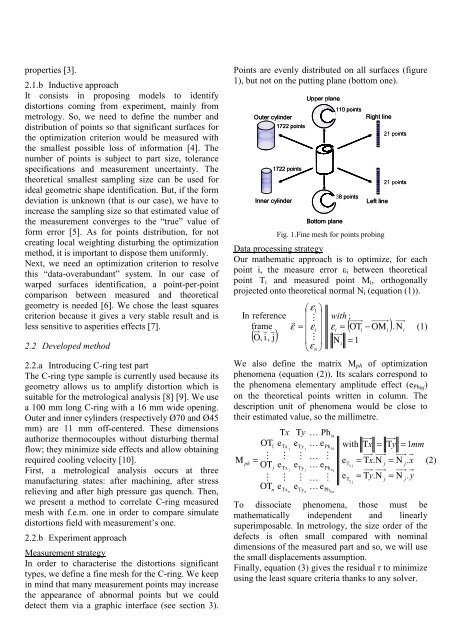
properties [3].2.1.b Inductive approachIt consists in proposing models to identifydistortions coming from experiment, mainly frommetrology. So, we need to define the number anddistribution of points so that significant surfaces forthe optimization criterion would be measured withthe smallest possible loss of information [4]. Thenumber of points is subject to part size, tolerancespecifications and measurement uncertainty. Thetheoretical smallest sampling size can be used forideal geometric shape identification. But, if the formdeviation is unknown (that is our case), we have toincrease the sampling size so that estimated value ofthe measurement converges to the “true” value ofform error [5]. As for points distribution, for notcreating local weighting disturbing the optimizationmethod, it is important to dispose them uniformly.Next, we need an optimization criterion to resolvethis “data-overabundant” system. In our case ofwarped surfaces identification, a point-per-pointcomparison between measured and theoreticalgeometry is needed [6]. We chose the least squarescriterion because it gives a very stable result and isless sensitive to asperities effects [7].2.2 Developed method2.2.a Introducing C-ring test partThe C-ring type sample is currently used because itsgeometry allows us to amplify distortion which issuitable for the metrological analysis [8] [9]. We usea 100 mm long C-ring with a 16 mm wide opening.Outer and inner cylinders (respectively Ø70 and Ø45mm) are 11 mm off-centered. These dimensionsauthorize thermocouples without disturbing thermalflow; they minimize side effects and allow obtainingrequired cooling velocity [10].First, a metrological analysis occurs at threemanufacturing states: after machining, after stressrelieving and after high pressure gas quench. Then,we present a method to correlate C-ring measuredmesh with f.e.m. one in order to compare simulatedistortions field with measurement’s one.2.2.b Experiment approachMeasurement strategyIn order to characterise the distortions significanttypes, we define a fine mesh for the C-ring. We keepin mind that many measurement points may increasethe appearance of abnormal points but we coulddetect them via a graphic interface (see section 3).Points are evenly distributed on all surfaces (figure1), but not on the putting plane (bottom one).Outer cylinder1722 points1722 pointsInner cylinderUpper planeBottom plane110 pointsRight line38 pointsLeft lineFig. 1.Fine mesh for points probing21 points21 pointsData processing strategyOur mathematic approach is to optimize, for eachpoint i, the measure error ε i between theoreticalpoint T i and measured point M i , orthogonallyprojected onto theoretical normal N i (equation (1)).⎛ ε1⎞⎜ ⎟ with :r M⎜ ⎟r ε = εiεi= ( ΟΤi− ΟΜi).Νi(1)⎜ ⎟⎜ M ⎟ Νi= 1⎝εn ⎠In referenceframer( Ο,i, j)We also define the matrix M ph of optimizationphenomena (equation (2)). Its scalars correspond tothe phenomena elementary amplitude effect (e Phnj )on the theoretical points written in column. Thedescription unit of phenomena would be close totheir estimated value, so the millimetre.ΜphΤxΤyK PhΟΤ1eTxeTyK ePh1 1=ΟΤMjeMTxeMej TyK K Mj PhΟΤM eMeMKKeMnTxnTynPhnn1n jnnwith Τx=eeTTx jy j= Τx.Ν= Τy.ΝjjΤy= 1mm= Ν . x= Ν . yTo dissociate phenomena, those must bemathematically independent and linearlysuperimposable. In metrology, the size order of thedefects is often small compared with nominaldimensions of the measured part and so, we will usethe small displacements assumption.Finally, equation (3) gives the residual r to minimizeusing the least square criteria thanks to any solver.jj(2)