Brayton Cycle Experiment – Jet Engine - Turbine Technologies

OBJECTIVE
Brayton Cycle Experiment – Jet Engine
1. To understand the basic operation of a Brayton cycle.
2. To demonstrate the application of basic equations for Brayton cycle analysis.
BACKGROUND
The Brayton cycle depicts the air-standard model of a gas turbine power cycle. A simple gas turbine is
comprised of three main components: a compressor, a combustor, and a turbine. According to the
principle of the Brayton cycle, air is compressed in the compressor. The air is then mixed with fuel,
and burned under constant pressure conditions in the combustor. The resulting hot gas is allowed to
expand through a turbine to perform work. Most of the work produced in the turbine is used to run
the compressor and the rest is available to run auxiliary equipment and produce power. The gas
turbine is used in a wide range of applications. Common uses include stationary power generation
plants (electric utilities) and mobile power generation engines (ships and aircraft). In power plant
applications, the power output of the turbine is used to provide shaft power to drive a generator, a
helicopter rotor, etc. A jet engine powered aircraft is propelled by the reaction thrust of the exiting gas
stream. The turbine provides just enough power to drive the compressor and produce the auxiliary
power. The gas stream acquires more energy in the cycle than is needed to drive the compressor. The
remaining available energy is used to propel the aircraft forward.
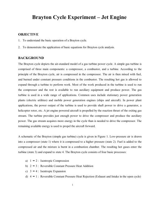
A schematic of the Brayton (simple gas turbine) cycle is given in Figure 1. Low-pressure air is drawn
into a compressor (state 1) where it is compressed to a higher pressure (state 2). Fuel is added to the
compressed air and the mixture is burnt in a combustion chamber. The resulting hot gases enter the
turbine (state 3) and expand to state 4. The Brayton cycle consists of four basic processes:
a) 1 � 2 : Isentropic Compression
b) 2 � 3 : Reversible Constant Pressure Heat Addition
c) 3 � 4 : Isentropic Expansion
d) 4 � 1 : Reversible Constant Pressure Heat Rejection (Exhaust and Intake in the open cycle)
1

CYCLE ANALYSIS
k
j
Atmospheric
Air
W &
Figure 1. Basic Brayton Cycle
in
Qin &
Combustor
Thermodynamics and the First Law of Thermodynamics determine the overall energy transfer. To
analyze the cycle, we need to evaluate all the states as completely as possible. Air standard models are
very useful for this purpose and provide acceptable quantitative results for gas turbine cycles. In these
models the following assumptions are made.
1. The working fluid is air and treated as an ideal gas throughout the cycle;
2. The combustion process is modeled as a constant-pressure heat addition;
3. The exhaust is modeled as a constant-pressure heat rejection process.
In cold air standard (CAS) models, the specific heat of air is assumed constant (perfect gas model) at
the lowest temperature in the cycle. The effect of temperature on the specific heat can be included in
the analysis at a modest increase in effort. However, closed form solutions would no longer be
possible.
2
l
Compressor Turbine
Hot
Exhaust
m
W &
output

To perform the thermodynamic analysis on the cycle, we consider a control volume containing each
component of the cycle shown in Figure 1. This step is summarized below.
Compressor
Consider the following control volume for the compressor,
Figure 2. Compressor Control Volume Model
Note that ideally there is no heat transfer from the control volume (C.V.) to the surroundings. Under
steady-state conditions, and neglecting the kinetic and potential energy effects, the first law for this
control volume is then written as
H�
− W = H
(1)
in
�
in
�
out
Considering that we have one flow into the control volume and one flow out of the control volume,
we may write a more specific form of the first law as
m� hin
− m�
wC
= m�
hout
(2)
Or, rearranging by grouping the terms associated with each stream,
− w
C = hout
- hin
This is the general form of the First Law for a compressor. However, if the fluid stream is assumed
to ideal gases we may represent the enthalpies in terms of temperature (a much more measurable
quantity) by using the appropriate equation of state ( dh = c pdT ), which will introduce the specific
Assuming constant specific heats, enthalpy differences are readily expressed as temperature
differences as
− w
C
= c
p.C
( T - T )
C, out
C.V.
C, in
Compressor
3
€
ó
(3)
(4)

To be more accurate, the specific heat of each fluid should be evaluated at the linear average between
⎛ Tin + Tout
⎞
its inlet and outlet temperature, ⎜ ⎟ .
⎝ 2 ⎠
The irreversibilities present in the real process can be modeled by introducing the compressor
efficiency,
η
COMP
w
=
w
C, s
C, a
=
h
h
out, s
out, a
- h
- h
in
in
where the subscript s refers to the ideal (isentropic) process and the subscript a refers to the actual
process. For a perfect gas the above equation is reduced to
η
COMP
Combustor
For the combustor,
=
T
T
out, s
out, a
- T
- T
in
in
Figure 3. Combustor Control Volume Model
Note that ideally there is work transfer from the control volume (C.V.) to the surroundings. Under
steady-state conditions, and neglecting the kinetic and potential energy effects, the first law for this
control volume is then written as
H�
+ Q = H
(7)
in
�
in
�
out
C.V.
Combustor
ó
Considering that we have one flow into the control volume and one flow out of the control volume,
we may write a more specific form of the first law as
m� hin
+ m�
qC
= m�
hout
(8)
4
ì
(5)
(6)

Or, rearranging by grouping the terms associated with each stream,
q
B = hout
- hin
Assuming ideal gases with constant specific heats, enthalpy differences are readily expressed as
temperature differences as
q
B
= c
p.B
( T - T )
B, out
B, in
Again, to be more accurate, the specific heat of each fluid should be evaluated at the linear average
between its inlet and outlet temperature.
Turbine
Consider the following control volume for the turbine,
Figure 4. Turbine Control Volume Model
Note that ideally there is no heat transfer from the control volume (C.V.) to the surroundings. Under
steady-state conditions, and neglecting the kinetic and potential energy effects, the first law for this
control volume is then written as
in
�
out
�
out
5
(9)
(10)
H�
− W = H
(11)
Considering that we have one flow into the control volume and one flow out of the control volume,
we may write a more specific form of the first law as
m� hin
− m�
wT
= m�
hout
(12)
Or, rearranging by grouping the terms associated with each stream,
− w
T = hout
- hin
C.V.
Turbine
ì
ö
(13)

Assuming ideal gases with constant specific heats, enthalpy differences are readily expressed as
temperature differences as
− w
T
= c
p.T
( T - T )
T, out
T, in
As before, the specific heat of each fluid should be evaluated at the linear average between its inlet
and outlet temperature for more accurate results.
The irreversibilities present in the real process can be modeled by introducing the turbine isentropic
efficiency,
wC,
a hout,
a - hin
ηTURB
= =
wC,
s hout,
s - hin
(15)
where the subscript s refers to the ideal (isentropic) process and the subscript a refers to the actual
process. For a perfect gas the above equation is reduced to
η
TURB
=
T
T
out, a
out, s
- T
- T
in
in
EXPERIMENTAL SETUP
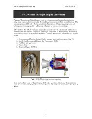
The laboratory setup is a self-contained, turnkey and portable propulsion laboratory manufactured by
Turbine Technologies Ltd. called TTL Mini-Lab. The Mini-Lab consists of a real jet engine.
Therefore, the same safety concerns of running a jet engine are present. Care must be taken to follow
all the safety procedures precisely as outlined in the laboratory and stated by your lab instructors. The
following description of the setup is provided by the manufacturer.
“A Turbine Technologies Model SR-30 turbojet engine is the systems primary
component. Operational sound and smell are hard to distinguish from any idling,
small business jet. The engine’s axial turbine wheel and vane guide ring are vacuum
investment castings. They are produced from modern, high cobalt and nickel
content super alloys (MAR-M-247 and Inconnel 718). The combustion chamber
consists of an annular, counterflow system, including internal film cooling strips.
Fuel and oil tanks, filters, oil cooler, all necessary plumbing and wiring is located in
the lower part of the Mini-Lab structure. A throttle lever is located on the right side
of the operator and above the slanted instrument panel. The throttle enables the
6
(14)
(16)

operator to perform smooth power changes between idle and maximum N1. Digital
engine RPM and E.G.T. gauges, mechanical E.P.R., Oil, Fuel, Air start pressure
gauges are also part of the standard panel. Annunciator lights indicate low oil
pressure, ignitor on, and air-start status. A key operated master switch controls the
main electric power bus. Other panel-mounted switches control igniter, air start, and
activate fuel flow. The SR-30 engine’s fuel system is very similar to large-scale
engines—fuel atomization via 6 return flow high-pressure nozzles that allow
operation with a wide variety of kerosene based liquid fuels (e.g. diesel, Jet A, JP-4
through 8).”
Figure 5. Turbine Technologies’s “MiniLab” Engine
Engine Components.
The engine consists of a single stage radial compressor, a counterflow annular combustor and a single
stage axial turbine which directs the combustion products into a converging nozzle for further
expansion. Details of the engine may be viewed from the ‘cutaway’ provided in Fig. 6.
7

Instrumentation.
The sensors are routed to a central access panel and interfaced with data acquisition hardware and
software from National Instruments. The manufacturer provides the following description of the
sensors and their location.
“The integrated sensor system (Mini-Lab) option includes the following probes:
Compressor inlet static pressure (P ), Compressor stage exit stagnation pressure
1
(P ), Combustion chamber pressure (P ), Turbine exit stagnation pressure (P ),
02 3 04
Thrust nozzle exit stagnation pressure (P ), Compressor inlet static temperature
05
(T ), Compressor stage exit stagnation temperature (T ), Turbine stage inlet
1 02
stagnation temperature (T ), Turbine stage exit stagnation temperature (T ), and
03 04
thrust nozzle exit stagnation temperature (T ). Additionally, the system includes a
05
fuel flow sensor and a digital thrust readout measuring real time thrust force based
upon a strain gage thrust yoke system.”
Figure 6. Turbine Technologies’s SR-30 Engine
Cut Away View of SR-30 Engine
8

EXPERIMENTAL PROCEDURE
SAFETY NOTES:
1. Make sure you are wearing ear protection. If you are not sure how the
earplugs are properly used, ask you lab instructor for a demonstration.
Never stay in the laboratory without ear protection while the engine is in
operation.
2. The SR-30 engine operates at high rotational speeds. Although there is a
protective pane that separates the engine from the operator, make certain
that you do not lean too close to this pane.
3. Make sure the low-oil-pressure light goes off immediately after an
engine start. If it stays on or comes on at any time during the engine
operation cut off the fuel flow immediately.
4. There is a vibration sensor whose indicator is to the far right of the
operator’s panel. If this indicator shows any activity (increase in voltage)
shut-off the engine immediately.
5. If at any time you suspect something is wrong shut off the fuel
immediately and notify the lab instructor.
6. If the engine is hung (starts but does not speed up to idle speed of about
40,000 rpm) turn the air-start back on for a short while until the engine
speeds up to about 30,000 rpm. Then turn off the air-start switch.
� MAKE SURE NEITHER YOU NOR ANY OF YOUR BELONGINGS
ARE PLACED IN FRONT OF THE INTAKE TO OR EXHAUST FROM
THE ENGINE WHEN THE ENGINE IS RUNNING.
9

1. Ask your TA to load the data acquisition program and run the pre-programmed LabView VI for
this lab. The screen should display readings from all sensors. Review the readouts to make sure
they are working properly.
2. Make sure that the air pressure in the compressed-air-start line is at least 100 psia (not exceeding
120 psia). Ask your lab instructor to check the oil level.
3. Make the appropriate length measurements and record the required dimensions so you can
calculate the inlet area (where the sensors are).
4. Ask the help of your lab instructor turn on the system and start the engine. After the engine is
successfully started, you must first allow the engine to achieve the idle speed before making any
measurements. Make sure the throttle is at its lowest point. The idle position is nearly vertical,
and is close to the operator (away from the engine).
5. Slowly open the throttle. Start taking data at about 65,000 rpm. Make sure that you allow the
engine time to reach steady state by monitoring the digital engine rpm indicator on panel. The
reading fluctuates somewhat so use your judgement.
6. Take data at three different engine speeds. You will use the data to study how cycle and
component efficiencies change with speed.
7. After you are done taking data, turn off the fuel flow switch first.
8. The data will be stored in Excel spreadsheet format
DATA ANALYSIS
Using the collected data determine the turbine isentropic efficiency, compressor isentropic efficiency,
the thermal efficiency of the cycle and the corresponding Carnot efficiency.
REPORT
In your report determine the performance of the ideal cycle operating with the same maximum cycle
temperature, mass flow rate, and compression ratio. Compare the performance of the ideal cycle
with measured performance. Discuss the differences.
SUGGESTIONS FOR DISCUSSION
1. How does the cycle efficiency compare with the ideal Brayton cycle? with the Carnot cycle?
2. How does the component efficiency affect the cycle efficiency?
3. How do the component efficiencies you calculated based on your test data compare with those of
typical of those gas turbine engines?
10