T - IfB

Monte Carlo MethodsNicholas ConstantineMetropolisStanislaw Ulam1Books about Monte Carlo• M.H. Kalos and P.A. Whitlock: „Monte CarloMethods“ (Wiley-VCH, Berlin, 2008 )• J.M. Hamersley and D.C. Handscomb:„Monte Carlo Methods“ (Wiley & Sons, N.Y.,1964)• K. Binder and D. Heermann: „Monte CarloSimulations in Statistical Physics“ (Springer,Berlin, 1992)• R.Y. Rubinstein: „Simulation and the MonteCarlo Method“ (Wiley & Sons, N.Y., 1981)2

Monte Carlo Method (MC)Simulates an experimental measuring processwith sampling and averaging.Big advantage:Systematic improvement by increasingthe number of samples N.Error goes like:1N3Applications of Monte Carlo• Statistical partition functions,i.e. averages at constanttemperature• High dimensional integrals4

Calculation of π1x 2 + y 2 = 1 124 1x dx001Choose N pairs(x i , y i ) , i = 1,…,Nof random numbersx i ,y i {0,1}5Calculation of πc = 0ific is number of points that fall inside circle.applety 1x c c12 2iarea c / N( N ) ( N) 41NcN6

Calculation of integralsg(x)baax iN 1 gxdx ( ) ( ba) gx (i)N i 1 b7Calculation of integralsrandom numbers x i [a,b]homogeneously distributed:„simplesampling“Good if g(x) smooth.8

Error of integrationconventional method:choose N equidistant points distanceone dimensionareahbNwhere T is thecomputer time.error:a1 1N T2h 2 2Δ (N area) 2 T -29Error in d dimensionsin d dimensions:1 1h , T N L d dhTLerror with conventional method:22d 2 2( d1)d Nhh T h Terror with Monte Carlo:1N Monte Carlo better for d > 4T1210

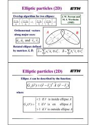
High dimensional integralConsider n hard spheres of radius R in a 3d3box.Phase space is 3n dimensional: (x(i , y i , z i ), i = 1,…,n.r ( x x ) ( y y ) ( z z)2 2 2ij i j i j i jwith hard sphere constraint( x x ) ( y y ) ( z z ) R2 2 2ijijij2Calculate average distance:1 2r r dx ,.., dx dy ,.., dy dz ,.., dzij ij 1 n 1 n 1 nZ nn ( 1)ij11MC strategy• Choose particle position.• If the excluded volume condition isnot fulfilled then reject.• Once the n particles are placed,calculate the average of r ij over allpairs (i,j).12

Not smooth integralsg(x)ax ineed more precisionb13Calculation of integralsgx ( )1 gx (i)g( x) dx p( x) dx ( b a)px ( ) N px ( )b b Naai1iif x i randomly distributed according to p(x).Good convergence when functiong( x)px ( )smooth.„importancesampling“14

Canonical Monte CarloE(X) ) = energy of configuration XProbability for system to be in X is given byBoltzmann factor:Z T is the partition function:1peq( X) eZTE( X )kTZTXE( X )kTe p ( ) eqX 1X15Problem of samplingQT ( ) Q( X) peq( X)XThe distribution ofenergy E aroundthe average < E > Tgets sharper withincreasing size.Choosing configurations equally distributedover energy would be very ineffective.16

M(RT) 2 algorithmN.C. Metropolis, A.W. Rosenbluth,M.N. Rosenbluth, , A.H. Teller and E. Teller (1953)importance sampling through a Markov chain:X 1 X 2 …..where the probability for a configuration is p eq (X)Markov chain: X t only depends on X t -1Properties of Markov chainStart in configuration X and propose a newconfiguration Y with probability T (XY).1. Ergodicity: One must be able to reach anyconfiguration Y after a finite number of steps.2. Normalization:3. Reversibility:YT( X Y)1T( X Y) T( Y X)1718

Transition probabilityThe proposed configuration Y will beaccepted with probability A(XY) .Total probability of Markov chain is:W(XY) ) = T(XY) A(XY)Master equation:dp( X , t)dt YpYW ( ) ( Y X) p( XW ) ( X Y)Y19Properties of W(XY)• Ergodicity:XY , : W( XY)0• Normality:• Homogeneity:YW( X Y)1 pst( Y) W( Y X) pst( X)Y20

Detailed balancedp( X , t)dt pY ( ) W( Y X) p( X) W( XY)YIn stationary state one should haveequilibrium distribution (Boltzmann)dpst( X , t)0dtY, p ( X) p ( X) p ( Y) W( Y X) p ( X) W( X Y)Yeqstsufficient condition is detailed balance:p ( Y) W( Y X) p ( X) W( X Y)eqYeqeqeq21Metropolis (M(RT) 2 ) peq( Y)AX ( Y) min1,peq( X) Boltzmann:1peq( X) eZTE( X )kTE( Y) E( X)EkTkTAX ( Y) min( 1, e ) min( 1, e )decreasesIf energy always acceptEincreases accept with probability .e - kT22

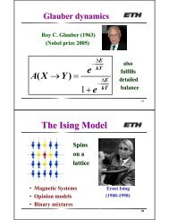
Glauber dynamicsRoy C. Glauber (1963)(Nobel prize 2005)AX ( Y)eEkT1eEkTalsofulfillsdetailedbalance23The Ising ModelSpinson alattice• Magnetic Systems• Opinion models• Binary mixturesErnst Ising(1900-1998)1998)24

The Ising ModelBinary variables:i1, i 1,...,Non a graph of N sitesinteracting via the Hamiltonian:HN E J Hi, j:nnNi j ii125Order parameterspontaneous magnetization:MN1( T ) lim iH 0Ni1M( T T)cordered phasedisordered phasecriticaltemperatureβ = 1/8 (2d)β ≈ 0.326 (3d)26

Susceptibility(T )TTcγ = 7/4 (2d)γ ≈ 1.24 (3d)numerical data from a finite systemMC of the Ising ModelSingle flip Metropolis:new configurationold configuration• Choose one site i (having spin σ i ).• Calculate ΔE = E(Y) -E(X) = 2Jσ i h i .• If ΔE < 0 then flip spin: σ i → - σ i .• If ΔE > 0 flip with probability exp(-ΔE/kT).27where h i is the local field at site iapplethi nn of ij28

Binary mixtures(lattice gas)Consider two species A and B distributed withgiven concentrations on the sites of a lattice.E AA is energy of A-A A A bond.E BB is energy of B-B B B bond.E AB is energy of A-B A B bond.Set E AA = E BB = 0 and E AB = 1.Number of each species is constant.29Kawasaki dynamics• Choose any A-B bond.• Calculate ΔE for A-B → B-A.• Metropolis: If ΔE ≤ 0 flip, elseflip with p = exp(-βΔE).• Glauber: Flip with probabilityp = exp(- βΔE)/(1+ exp(- βΔE)).β = 1/kTKyozi Kawasaki30

Interfaces31InterfacesABsurface tension fA+BfA32

Ising interface+++ +NH E J ij+i, j:nn+++Fixed boundary conditions:upper half „+“,, lower half „–“hSimulate with Kawasakidynamics at temperature T.----- - --Ising interfaceinterface width W:33W1Nh 2ihiWTT croughening transition34

Self-affine scalingFamily-Vicsek scaling (1985):L t L f z t L W , /ξ is the roughening exponent, z the dynamic exponent.35Self-affine scaling zLt L f t LW , /u t/Lzt :WL f u L:W t f u 0u z zW Lu L t/L L t const is the growth exponent. Numerically these laws are verified by data collapse.0z36

Ising interfaceAdd next-nearest nearest neighbor interaction:HN E J K i j i ji, j: nni, j:nnnNpunishes curvature introduces stiffness+_+_11 K17 K37Shape of drop• Start with a block of +1 sites attached to wall ofan LL system filled with -1.• Hamiltonian including gravity g:HwithN E J K h Ni j i j j ii, j: nn i, j:nnn j line j( j1)( hLh)h hhjh1 and g L 1L1 L 1• Use Kawasaki dynamics and further do not allowfor disconnected clusters of +1.38

Shape of dropL = 257, V = 6613, g = 0.001after 51057 MC updatesaveraged over 20 samples.Contact angle θ is functionof temperature and vanisheswhen approaching T c .θ39Solid on solid model (SOS)adatoms andsurface growthinterface without islands and without overhangsHN E h hi, j:nnij40

Irreversible growth• T. Vicsek, „Fractal Growth Phenomena“(World Scientific, Singapore, 1989• A.-L. Barabasi and H.E. Stanley, „FractalConcepts in Surface Growth“ (CambridgeUniv. Press, 1995)• H.J. Herrmann, „Geometric ClusterGrowth Models and Kinetic Gelation“,Phys. Rep. 136, 153 (1986)41Irreversible growthNo thermal equilibrium• Deposition and aggregation patterns• Fluid instabilities• Electric breakdown• Biological morphogenesis• Fracture and Fragmentation42

Random deposition43Random depositionsimplest possible growth modelPick a random column.Add a particle on top ofthat column = 1/2ξ = 1/2hW~ t~t1/244

Random deposition with surface diffusionParticle can move a short distance to find amore stable configuration.Pick a random column i.Compare h(i) and h(i+1).Particle is added onto whichever is lower. Ifthey are equal, add to column i or i+1 withequal probability. = 1/4ξ = 1/2hW~ t~t1/445Restricted Solid On Solid Model (RSOS)Neighbouring sites may not have a heightdifference greater than 1.Pick a random column i.Add a particle only ifh(i) h(i-1) and h(i) h(i+1).Otherwise pick a new column. = 1/3ξ = 1/2c46

Eden modelsimple model for tumor growth or epidemic spreadEach site that is a neighbour of an occupied sitehas an equal probability of being filled.Make a list of neighbour sites (red).Pick one at random. Add it to cluster (green).Neighbours of this site then become red….There can be more than one growth site in acolumn. Can get overhangs.c47Eden cluster = 1/3ξ = 1/248

Ballistic depositionParticles fall vertically from above andstick when they touch a particle below or aneighbour on one side.Pick a column i. Let particle fall till ittouches a neighbour. Possible growth sitesare indicated in red. Only one possible siteper column.c = 1/3ξ = 1/249KPZ equation:Growth equationsEdwards Wilkinson equation: hxt( , )tS.F. Edwards and D.R. Wilkinson (1982) = 1/4 and ξ = 1/2h( x, t)hxt( , ) h h 2( x, t)t2M. Kardar, G. Parisi and Y.-C. Zhang (1986) = 1/3 and ξ = 1/2noise50

Diffusion Limited Aggregation (DLA)A particles starts a long wayfrom surface.It diffuses until it firsttouches the surface. If itmoves too far away, anotherparticle is started.c51Electrodeposition52

DLA clustersfractaldimensiond f = 1.7(in 2d)53Viscous Fingering54

DLA clustersanisotropy on square lattice:55Scale Invariance56

Dielectric breakdown57Dielectric breakdown model (DBM)Solve Laplacian field ϕ:p 0and occupy siteat boundarywith probability:same as DLAη = 158

Dielectric breakdown modelη = 459Dielectric breakdown modelη = 260

Dielectric breakdown modelη = 0.161Dielectric breakdown modelsame as Eden modelη = 062

Clustering of clustersFractal dimension is d f ≈ 1.42 in 2d, d f ≈ 1.7 in 3d.dynamical scaling:2zns s f s/twith dynamical exponent z .Simulated Annealing63• P.J.M. Van Laarhoven and E.H. Aarts,„Simulated Annealing: Theory andApplications“ (Kluwer, 1987)• A. Das and B.K. Chakrabarti (eds.),„Quantum Annealing and RelatedOptimization Methods“ Lecture Notes No.679 (Springer, 1990)64

Simulated Annealing (SA)S. Kirckpatrick, C.D. Gelatt and M.P. Vecci, 1983SA is a stochastic optimization technique.Given a finite set S of solutionsand a cost function F: S Search a global minimum:s* S* { s S : F(s) F(t) t S }.Difficult when S is very big (like |S| = n!).65Travelling SalesmanGiven n cities σ i and the travelling costs c(σ i ,σ j ).We search for the cheapest trip through allcities.• S = { permutations of {1,..,n} }• F() = i=1..n c(σ i ,σ j ) für SFinding the best trajectory is a NP-complex problem,i.e. time to solve grows faster than any polynomial of n.66

Travelling SalesmanMake local changes: Define close configuration on SN : S 2 S with i N(j) j N(i)(i)´ N() j i j(j) ´iTraditional optimization algorithm:Improove systematically the costs by exploring close solutions.If F(σ´) < F(σ) replace σ σ ´ until F(σ) F(t) for all t N(σ).Problem: One gets stuck in local minima.Travelling SalesmanSimulated annealing optimization algorithm:If F(σ´) < F(σ) replace σ σ ´If F(σ´) > F(σ) replace σ σ ´with probability exp(- F / T)with F= F(σ ´)-F(σ ) > 0T is a constant (like a temperature)Go slowly to T 0 in order to find global minimum.67Applet68

Slow coolingT 0T 1T 20Different cooling protocols are possible.Asymptotic convergence is guarantied andleads to an exponential convergence time.69Lattice gas• D.H. Rothman and S. Zaleski, „Lattice-GasCellular Automata“ (Cambridge Univ.Press, 1997)• J.-P. Rivet and J.P. Boon, „Lattice GasHydrodynamics“ (Cambridge Univ. Press,2001)• D.A. Wolf-Gladrow, „Lattice-Gas CellularAutomata and Lattice Boltzmann Models“(Lecture Notes, Springer, 2000)70

Lattice gasParticles move on a triangular lattice andfollow the following collision rules:Momentum is conserved at each collision.It can be proven (Chapman-Enskog) thatits continuum limit is the Navier Stokes eq.71von Karman streetvelocity field of a fluid behind an obstacleEach vector is an average over time and space.72

Solving equationsFinding the solution (root)) of an equation:f (x)) = 0is equivalent to the optimization problemof finding the minimum (ormaximum) ) of F(x)given by:d F ( x )dx073Newton methodBe x 0 a first guess, then linearize around x 0 :f( x ) f( x ) ( x x ) f '( x ) 01 0 1 0 0xx n1nf( x )fn'( x )n74

Secant methodIf derivative of f is not known analytically:ff( x ) f( x )n n1'( xn) xn xn1x x ( x x)n1 n n n1f( x )nf( x ) f( x )nn175Secant method76

Bisection methodTake two starting values x 1 and x 2with f (x 1 ) < 0 and f (x 2 ) > 0.Define mid-pointx m as x m = (x(1 + x 2 ) / 2 .If sign(f (x m )) = sign(f (x 1 ))then replace x 1 by x motherwise replace x 2 by x m .77Bisection method78

Regula falsiTake two starting values x 1 and x 2with f (x 1 ) < 0 and f (x 2 ) > 0.Approximate f by a straight line betweenf (x 1 ) and f (x 2 ) and calculate its root as:x m = (f((x 1 ) x 2 – f (x 2 ) x 1 ) / (f (x 1 ) – f (x 2 )).If sign(f (x m )) = sign(f (x 1 )), thenreplace x 1 by x m otherwise replace x 2 by x m .Regula falsi7980

N-dimensionalequationsBex a N-dimensionalvector.System of N coupled equations:f( x)0corresponding to the N-dimensionaloptimization problem: ( x F ) 081N-dimensional Newton methodJDefine the Jacobi matrix:i,j fi( x)( x) xjMust be non-singularandalso well-conditionedfor numerical inversion. x x J f ( x )1n 1 n n82

System of linear equationsb 11 x 1 +. . . . + b 1N x N = c 1. . . . . .. . . . . .b N1 x 1 + . . . + b NN x N = c N Bxcsolution:x B1c83System of linear equations f( x) Bxc 0J Bapply Newton method:x x B1 ( Bx c)B1cn1 n n exact solution in one step x x J f x 1( )n1n n84

N-dimensionalsecant methodIf the derivatives are not known analytically:Ji,j( x) f ( xh e ) f ( x)i j j ihjwhere h j should be chosen as:being ε the machine precision,i.e. ≈ 10 -16for a 64 bit computer.h xj j85Other techniquesRelaxation method: f ( x) 0 x g ( x , j i), i 1,...,Ni i jStart with x i (0) and iterate: x i (t+1) = g i (x j (t)).Gradient methods:1. Steepest descent2. Conjugate gradient86

Ordinary differential equationsFirst order ODE, initial value problem:dydt f ( yt , )with y (t 0 ) = y 0examples:radioactive decaycoffee coolingdTdtdNdtN( T T)room87Euler methodexplicit forward integration algorithmchoose small Δt, , Taylor expansion:dy2y( t0 t) y( t0) t ( t0) O( t)dt y t f( y , t ) O( t) y( t ) y20 0 0 1 1convention:tn t0 nt , yn y( tn)88

Euler methodStart with y 0 and iterate:y y t f y t O t 2n1 n(n,n) ( )This is the simplest finite difference method.Since the error goes with Δ 2 t one needs a verysmall Δt and that is numerically very expensive.Euler method8990

The Newton equationm2d x F ( x )2dt2nd order ODETransform in asystem of twocoupled ODEsof first order.dxdtdvdtvF( x)m91Euler method for N coupled ODEsN coupled ODEsof first order:dydtif ( y ,..., y , t) , i ,..., Ni1 N1iterate with a small Δt :y t y t t f y t y t t O t2i( n1) i( n) i( 1( n),..., N( n), n) ( )witht t ntn092

The order of a methodIf the error at one time-stepis O(Δ n t) themethod is „locallyof order n“. . To consider afixed time interval T one needs T /Δt time-stepsso that the total error is:T O t O ttnn1( ) ( )and therefore the method is „globallyof order n-1“.The Euler method is globally of first order.93Runge - Kutta method94

References for R-K method• G.E. Forsythe, M.A. Malcolm and C.B. Moler, „ComputerMethods for Mathematical Computations“ (Prentice Hall,Englewood Cliffs, NJ, 1977), Chapter 6• E. Hairer, S.P. Nørsett and G. Wanner, “Solving OrdinaryDifferential Equations I” (Springer, Berlin, 1993)• W.H. Press, B.P.Flannery, S.A Teukolsky and W.T. Vetterling,“Numerical Recipes” (Cambridge University Press, Cambridge,1988), Sect. 16.1 and 16.2• J.C. Butcher, „The Numerical Analysis of Ordinary DifferentialEquations“ (Wiley, New York, 1987)• J.D. Lambert, „Numerical Methods for Ordinary DifferentialEquations“ (John Wiley & Sons, New York, 1991)• L.F. Shampine, „Numerical Solution of Ordinary DifferentialEquations“ (Chapman and Hall, London, 1994)952nd order Runge - Kutta methodExtrapolate using Euler methodto the value halfway, i.e. . at t + Δt / 2:1 1y ( t t) y ( t) tf( y ( t), t)i i i2 2Evaluate derivative in Euler method at this value:1 12 2y t t y t t f y t t t t O t3i( ) i( ) (i( ), ) ( )96

Fourth order Runge - Kuttak1tf( y , t )k tf( y k /2, t t/2)2 n 1k tf( y k /2, t t/2)3 n 2k tf( y k , t t)4 n 3nnnnnRK4ynk1k2k3k451 yn O( t)6 3 3 697RK4• k 1 is the slope at the beginning of the interval.• k 2 is the slope at the midpoint of the interval, usingslope k 1 to determine the value of y at the pointt n +Δt/2 using Euler method.• k 3 is again the slope at the midpoint, but nowusing the slope k 2 to determine the y-value.• k 4 is the slope at the end of the interval, with its y-value determined using slope k 3 .Then use Euler method withslopek 2k 2k k1 2 3 4698

q-stageRunge - Kutta methoditeration:y y tkn1n i ii1qwithi1k f( y t k , t t)i n ij j n ij1and α 1 = 0explicitimplicit:qk f( y t k , t t)i n ij j n ij199q-stageRunge - Kutta methodq = 1 is the Euler method(unique)Butcher array or Runge-Kuttatableau:2 21 3 31 32 .... q q1 q2 q,q1 .... 1 2 q1qresumes allparametersof the generalRunge-Kutta100

Example RK4Butcher array:its stage is: q = 40½½½ 0 ½1 0 0 11 1 1 16 3 3 6RK4 is of order p = 4 applet101Order of Runge - Kutta methodThe R-K method is of order p if:q( ) p1( ) ii ( )i1y t t y t t k O tOne must choose the α i , β ij and ω i for i,j [1,p] ] suchthat the left hand side = 0 in O(Δt m ) for all m ≤ p.Taylor expansion:1 df y t t y t t O tpm1mp1( ) ( ) ( )m1 m1m! dt y( t),t102

Order of Runge - Kutta method1 df qpm1m1iki tm1i1 m1m! dt y( t),tup to O(Δt p+1)Example q = p = 1:1 f( yn, tn) f( yn, tn)1 1 gives Euler method.Example q = p = 2:1 df1k12k2 fn t2 dt where index „n“ means „at (y(n ,t n )“.Example q = p = 2n1031 df 1 f f1k12k2 f t f t f2 dt n2 t ny nn n ninsertk1 f( yn, tn) fnk f( y t k , t t )2 n21 1 n2ff fnt21 fnt 2O ty t n 1 1 121, 22 , 2212 2n2( )3 equations for 4 parameters one-parameterfamily104

Example q = p = 2y ny t ( 1 ) k k1 n2 1 2 2k f( y , t )1nntt ( , )k2f yntn22 22105Order of Runge - Kutta methodTo obtain a Runge-Kuttamethod of givenorder p one needs a minimum stage of q min .p 1 2 3 4 5 6 7 8 9 10q min 1 2 3 4 6 7 9 11 12 – 17 13 - 17John Butcher106

Example: Lorenz equationIs a simplified system of equations describing the 2-dimensional2flow of fluid of uniform depth in the presence of an imposedtemperature difference taking into account gravity, buoyancy,thermal diffusivity, and kinematic viscosity (friction).σ Prandtl number Rayleigh numberσ = 10 , = 8/3 is varied.Chaos for = 28.'y =σ y - y1 2 1'y = y ρ -y -y2 1 3 2'y = y y - βy3 1 2 3Edward Norton Lorenz(1963)appletC.Sparrow: „The Lorenz Equations: Bifurcations, Chaosand Strange Attractors“ (Springer Verlag, N.Y., 1982)107Example: Lorenz equationChaotic solutions of theLorenz equation exist andare not numerical artefacts(14th math problem of Smale).Warwick Tucker(2002)108

Adaptive time-stepΔtδ expectedDefine the errorThen measure the realdefine a newtime-stepthrough:tyou want to accept.error andreal errorbecause δ Δt p+1.δ measuredexpectednewtold measured1p1109Error estimationLet us consider a method of order p, (error = ΦΔt p+1) .Be y 1 the predicted value for 2Δtand y 2 the predicted value making two steps Δt.Define error as δ = y 1 – y 2y1 2t O tyt ( 2t) y22t O t 2 2t O tp1 p2( ) ( )p1 p2( ) ( )p1 p1 p2( ) ( )110

Error estimationimprove systematically:2yt t y O t2 2example RK4:p2( ) 2 ( )p1ytt y Ot15p2( )2( )111Error estimationGeneral for two different time steps Δt 1 and Δt 2pp1y ytti O tii , 1,2ip p p pp1t 2t1 y t2 y p t1y p O titt1 2t y t yy O tpp2 p 1 pt 1t2p1p pit2 t1112

Richardson extrapolationCalculate forvarious Δt iand extrapolatey =limytt i 0i113Bulirsch - Stoer MethodExtrapolate with rational function:ykp0 p1tn ... pk tnt nm tn0q0 q1tn ...qm tnR. Bulirsch and J. Stoer, „Introduction toNumerical Analysis“ (Springer, NY, 1992)ttn , n2, 4, 6,8,12,16, 24,32, 48, 64,96,. ..nChoose k and m appropiately.y114

Predictor-correctorcorrector methodidea:yt ( t) yt ( ) tmake predictionusing Taylor:correct byinserting:f ( yt ( )) f( yt ( t))2implicit equationdyy t t y t t t O tdtP2( ) () () ( )ty tt y t f y t f y tt O t2CP3( ) () [ ( ()) ( ( ))] ( )Can be iterated by again inserting corrected value.3th order predictor-correctorcorrector115Predict through 3rd order Taylor expansion:2 2 3 3Pdy t d y t d y4( ) () () () () ( )2 3y t t y t t t t t O tdt 2 dt 6 dtP2 2 3dy dy d y t d y3( tt) () t t () t () t O( t)2 3dt dt dt 2 dtP2 2 32( ) ( ) ( ) ( )2 tt t t t O t2 3d y d y d y dt dt dtP3 3d y dt d y( tt) ( t)O( t)dt3 3116

3th order predictor- correctoruse equation:dy dtCP( tt) f( y ( tt))define error:correct:Procedurecan berepeated.Cdy dy ( tt) ( tt)dt dt y ( tt) y cCP0C2 2d y d y ( t t)c2 2 2 dt dt C3 3d y d y ( t t)c3 3 3 dt dt 5th order predictor- correctorPPPGear coefficients:c 0 = 3/8c 2 = 3/4c 3 = 1/6117Be r 0 ≡ y. Then one can define the time derivatives:Predictor:118

5th order predictor- corrector1st order eq.:drdt f(r) r f(r ) r r rC P C P1 0 1 12nd order eq.:Corrector:d rdt2C P C P f(r) r 2 22f(r 0) r r2 r2119Gear coefficients (1971)1st order equation:2nd order equation:120

Comparison of methodsΔtfor fixed number of iterations nVerlet4th5th6therrory n+1- y nPredictor - Corrector121Sets of coupled ODEsExplicit Runge Kutta and Predictor Correctormethods can be straightforwardly generalizedto a set of coupled 1st order ODEs:dydtif ( y ,..., y , t) , i ,..., Ni1 N1by inserting simultaneously all the valuesof the previous iteration.122

Stiff differential equationexample:'y ( t) 15 y( t) , t 0 , y(0) 1Euler:yt t yt t yt O t2( ) () 15 () ( )Becomes unstable if Δt not small enough:Use implicit method (Adams – Moulton):12 2y( t t) y( t) t f ( y( t), t) f ( y( t t), t t) O( t)123Stiff sets of equationsy ' () t K y() t f This system is called() t if matrixThis system is called „stiff“if matrix K has at least onevery large eigenvalue.y ' () t f ( y (),) t tThis system is calledThis system is called „stiff“ ifJacobi matrix has at leastone very large eigenvalue.example:y 998y 1998y'1 1 2y 999y 1999y'2 1 2y (0) 1 , y (0) 11 2Solve with withimplicit method.124