T - IfB

Guidance on Impact AssessmentsDocument Type: GuidanceRef: 33/08Date of Publication: 31 March 2008Target Audience: All stakeholdersOverview:This document provides guidance on Ofgem’s approach to conducting impactassessments. The guidance has been revised to take account of best practice as it hasdeveloped, for instance in relation to sustainability issues, and it sets out Ofgem'sapproach to cost-benefit analysis.Amongst other things, the guidance sets out the legislative background for producingimpact assessments and outlines the basic framework that Ofgem will normally follow inproducing them.Whilst impact assessments are not determinative of the final policy decision that wemake, they are a vital part of the policy-making process and provide a valuableframework for assessing the impact of important policy proposals.Office of Gas and Electricity MarketsPromoting choice and value for all gas and electricity customersContact name and details: Andy MacFaul, Head of Better RegulationTel: 020 7901 7083Email: andrew.macfaul@ofgem.gov.ukTeam: Corporate Affairs Division

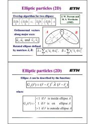
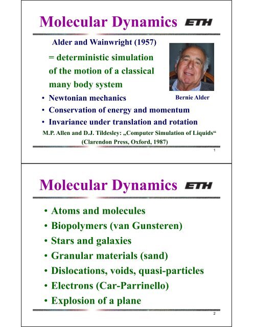
Molecular Dynamicsgeneralized coordinates with α degrees of freedomof particle i:N particles:Hamiltonianq q q p p p Q( q ,..., q ) , P( p ,..., p )1 1 i( i,..., i) ,i( i,..., i)1 N1H ( P, Q) K( P) V( Q)kinetic energy:K( P) m i is mass of particle i.k p 2i2mi k1iN3Potential energyMake expansion of potential energy VQ ( ) v( q) v( q, q) v( q, q, q) ...1 i 2 i j 3 i j ki i ji i ji kjTypically three or more body interactionsare neglected and their effect considered inan effective two body interactioneff attr rep v2 ( q , q ) v ( r) v ( r) , r q qi j i jattractiverepulsive4

Potentialshard core interaction 0.35 nm for atoms5elastic repulsionPotentialsr R R1 2for particles of radiusRandR1 2RRRR6

Potentialssoft core repulsion 1 electrostatics and gravity =12 soft repulsion7Potentialssquare potentialronly forces atandr 1 28

PotentialsLenard Jones potentialε is attractive energyσ is interaction range9Equations of motionHamilton equation:k Hk Hqi , pi , k 1,..., , i 1,...,Nkkpqii qi xi , qivi, i 1,...,N p ix ivi , piiV( Q) fimi mx f fi i i ijjvectorial sum of allforces acting on i10

Conservation laws• Energy conservation (as long as K(P) andV(Q) do not explicitely depend on time)• Momentum conservation (if system has nowalls) P pi• Conservation of angular momentum (ifsystem is spherical) L x piiii11Contact timer max is the turning point of a colliding particle,r min is the maximum range of the potential.12

Contact timeone dimensionenergy:122E mr V r const() .velocity:drdt2mEV()r12contact time:1t2maxmaxdt 2tc2 dt 2 dr 2 EV( r) drdr m0c r rrminrmin1213Solving the equations• Euler method• Runge Kutta method• Predictor-Corrector method• Verlet method• Leap-frog methodspecial forNewton eqs.14

Verlet methodLoup Verlet (1967)Taylor expansion in time step Δt: 1xtt xt tvt t 2vt 1xtt xt tvt t 2vt 2( ) () () () ...2( ) () () () ...add the two equations real timeΔt ≈ t c /20from Newton equation xt t xt xt t txt 2( ) 2 ( ) ( ) ( )15Verlet methodCalculate for all i = 1,..., N particles :1xi()t f ij( t) , f ij( t) V rij( t)mInsert this in :ij x t t x t x t t t x t2i( ) 2 i( ) i( ) i( )withrmax1 2min12t E V()r dr10 m r16

Verlet method• One needs to store two time steps (t and t – Δt).• Calculate velocities through:vt () xt ( t) xt ( t)2t• Error is O(Δt 4 ), i.e. third order algorithm.• Problem is addition of terms O(Δt 0 ) and O(Δt 2 ).• Improve systematically including more orders.• Exact time reversal.17Leap frog methodR.W. Hockney (1970)Consider velocities at intermediate times:from Newton equation 1 1vt ( t) vt ( t) txt ( )2 2 1x( tt) x( t) t v( t t)2No addition of terms O(Δt 0 ) and O(Δt 2 ) anymore.18

Leap frog methodVerletLeap frog19Leap frog methodLeap frogEuler f( x( t))vt ( t)m vt ( t) vt ( ) tvt ( t) x( tt) x( t) t v( tt) f( x( t))vt ( t)m xt ( t) xt ( ) tvt( ) vt ( t) vt ( ) tvt ( t)20

Total energy21Small perturbationdivergence betweentwo trajectoriestotal energy22

Comparing methodsMore precisionfor smaller Δt.Precisiongiven by:VerletΔtδ 2EE24thCorrectorpredictor6th5thfixed numberof iterations23Addaptive time stepΔttrajectory of a particle:Define a requiredprecision δ req .Measure the actual precision δ meas .For a method oforder n set:1 nreq tnewtold meas24

TricksMost time consuming loop is calculation of forcebecause one must consult all pairs of particles,therefore it goes like N 2 .Instead of calculating:d 2r x xij i j 1 V r r f f r r2n2( n1)( ) i ( )i25Force calculationIf potential is not a very simple one thanuse look-up tables.For example for the Lenard – Jones potentialintroduce a cut-off at r c = 2.5σ.Then divide interval in K pieces with points:lk2(0, )kKr cr2cThen look-up table becomes:F( k) f lk26

Force calculationThe index k is calculated through:k Sx x x x S Kr i j i j1 with2[x] is the largest integer smaller than x.Use Newton – Gregory interpolation: with 2f( z) F( k) ( kzS) F( k1) F( k) z xi xjc27Verlet tablesDefine around each particle i a neighborhoodof radius r l > r c .Store all the coordinatesof the particles in thisneighborhood in thevector LIST whichr lr chas a length N·N u where N u is the averagenumber of particles in the neighborhood.28

Verlet tablesThe Verlet table LIST is a one-dimensional vectorin which all neighborhoods are sequentially stored.A second vector POINT[i] contains the index ofthe first particle in the neighborhood of i in LIST.Therefore the particles in the neighborhood of i are:LIST[POINT[i]],…,LIST[POINT[i+1]-1].The force is calculated by just going throughthis list to find all the neighbors of i, (i.e. N).29Verlet tablesEverynrl r tvcmaxtime steps the Verlet tablemust be renewed (n ≈ 10 – 20) where v max is thelargest velocity of a particle, since otherwiseparticles beyond a distance r l could reach r c .Renewal requires N 2 operations so that theentire algorithm still goes like O(N 2 ).30

Linked cell methodPlace above the system a grid of size M d sothat each cell is larger than 2r c .All particles that caninteract with particle ilie in the shaded region.MDonald Knuth(1973)31Linked cell methodSo on average one just needs to test N·3 d N/M dparticles therefore reducing the loop by (M/3) d .To find out which particle is in one cell one storesin a vector FIRST of length M d for each cell theindex of the first particle. If no particle is in cell jthen FIRST[j]=0. In a second vector LIST[i]of length N one stores for each particle i the indexof the next particle in the same cell. For the lastparticle in a cell we set LIST[i]=0.32

Linked cell methodexamplecell 1 cell 2FIRSTFIRST33Linked cell methodProgram to find all particles in cell i = 2:M[1]=ANF[i];FIRST [ i ] ;i=2;while(M[i-1]!=0){M[j]=LIST[M[j-1]]}When a particle flies from one cell to another, onecan renew the lists FIRST and LIST locally so thatno loop over all N is necessary algorithm is O(N).34

ParallelizationUse the cell structure to divide system amongthe processors. Cells on the border are sentto the neighboring processor using MPI.processor 1 processor 2 processor 335Cut-off of potentialsPotential jump at cut-off r c generates infinite forces.Therefore consider another potential that is 0 at r c .V( r) Vc for r rc with Vc V( rc)V () r 0 for r rcThe jump in force at r c can be removed by:V() r VV() r V ( rr ) for r r rrc 0 for r rc c cc36

MoleculesMolecules are composed of several atoms = particlesand each is subjected to forces. One can bind themtogether through the attractive part of their potentialbut that needs deep potentials to avoid them fallingapart and therefore is computationally expensive.Since forces inside molecules are at least one orderof magnitude larger than those between them onecan just keep bonds (and angles) fixed.37MoleculesThere exist several ways to implement fixeddistances (or angles) inside a molecule or anyother structure that couples degrees offreedom:• Imposing constraints using Lagrangemultipliers.• Describing structures as rigid bodies.38

Water molecule39Lagrange multipliersJ.P. Ryckaert, G. Ciccotti and H.J.C. Berendsen, 1977Let us just consider fixed bond lengths for adiatomic molecule (e.g. water).Atom i (i = 1,2,3) follows the equation:mx f gi i i iforces from other moleculesforces toimposeconstraints40

Lagrange multipliersConstraints that bonds have length d 12 and d 23 :rd2 212 12 12rd2 223 23 2300with rij r , r x xij ij i j 1 1 gk 12 xk 12 23xk 232 2 where λ 12 and λ 23are the yet undetermined Lagrange multipliers.g r , g r r , g r1 12 12 2 23 23 12 12 3 23 2341Lagrange multipliersExecute theVerlet algorithmin two steps:insert g i ! 2 fixi( tt) 2 xi( t) xi( tt) tmi ! 2 gixi( tt) xi( tt) tm x ( tt) x ( tt) t r ( t)! 2 121 1 12m1 x ( tt) x ( tt) t r ( t) t r ( t)! 2 23 2 122 2 23 12m2 m2 x ( tt) x ( tt) t r ( t)! 2 233 3 23m3i42

Lagrange multipliersObtain λ 12 and λ 23 by inserting theseexpressions into the constraint condition:x t tx t t dx t tx t t d2 21( ) 2( ) 122 22( ) 3( ) 2343Lagrange multipliersThis gives the following coupled quadratic eqs.: 1 1 x ( tt) x ( tt) t r ( t) t r ( t)d ! ! 2 2 2321 2 12 12 23 12m1 m2 m2 1 1 x ( tt) x ( tt) t r ( t) t r ( t)d ! ! 2 2 1222 3 23 23 12 23m2 m3 m2Solve them to get λ 12 and λ 23 then usethese λ 12 and λ 23 to calculate .x ( t+ Δt)i2244

Lagrange multipliersFirst solve terms in Δt 2 since they are linear in λ ij ,then insert into equations for Δt 4 terms to improveaccuracy. For molecules with n bonds one has tosolve a system of n coupled quadratic equations.In case one wants to fix an angle one can do this byadding one extra bond.Care must be taken in the caseof molecules like butane:To control rotation around C-C axis use for instance afour-body potential (Ryckaert and Bellemans, 1978) .45Example DNAStretchingof a DNAchainDNA chainmovingthrougha pore46

Example nano-gear47Constraint DynamicsUp to now: Interactions of atoms through forcesderived from potentials, and additionalconstraints.Consider rigid objects of finite volume (e.g. sandgrains) which normally one would like to describeby a hard core potential which in classical MDcannot be handled because of the infinite forces.Idea: Interactions fully determined by constraints!Contact dynamics typically for granular materialsand rocks, building blocks, etc.48

Contact Dynamics (CD)P. Lötstedt (1982)J.J. Moreau and M. Jean (1992)Jean Jacques MoreauContact Dynamics treats rigid particles and is goodfor long-lasting contacts as they occur in densepackings. At contacts one imposes constraint forcesthat prevent the penetration of particles.Advantage: Δt not related to duration of collision49Contact DynamicsNon-smooth dynamicsSignorini-Graph:perfect volumeexclusion (perfectlyrigid particles)First: no friction between particleswith relative tangential velocity v sconsidered (added later).Thus: only normal forces at contacts!ns50

Contact DynamicsNon-smooth dynamicsnSignorini-Graph:perfect volumeexclusion (perfectlyrigid particles)sCoulomb-Graph:friction betweenparticles with relativetangential velocity v ssnns51Contact DynamicsCollisions of rigid bodies give rise todiscontinuous velocities, thus higherorder schemes are not beneficial. extUse implicit Euler integration: Fi R 1 vi( t t) vi( t) Fi( t t)tmi r( t t) r( t) v ( t t)ti i iexternal contacti52

Example: two particles (1D)Matrix H transforms contactforces (loc) into particleforces, H T particle velocitiesinto relative velocities (loc).loc1n loc R2 RnextF1locv1 vT 1 vn v2 v1 ( 1,1) H v v 2 2 R R 1loc Rn 1 v21 v1 2m m m1 2HRlocnextF253Example: two particles (1D)Newton‘s equation in vectorial form:extd v1 1 R1 F1 ext dt v2 m R2 F2Use for contact quantities (transformation by H):locdv1 1n F1 1 ( 1,1) R R F Fdt m 1 m mmeff1 Fext ext2 F1m m/2extloc 1loc ext extn ext n 2 1F2 effeffective massloc. acceleration without contact forces54

Example: two particles (1D)The equation hastwo unknowns:dvdtlocn1 1 R FFm mlocext extn2 1Using the implicit Euler integration leads to relation:locR ( t t)nwheremeffef flocloc,freevn( t t) vn( t t)tloc,free loc 1 ext extvn( t t) vn( t) F2 F1tmUse the constraint (Signorini) as conditionto define the contact force Rlocn .55Example: two particles (1D)Graphical interpretation:Signorini condition at contact(d=0) can be re-formulated interms of the local velocity.locR nIntersect withlocloc,freelocvn( t t) vn( t t)Rn( t t) mefftIllustrates solutions for persisting contactand opening contact.locv n56

Example: two particles (1D)No overlap (after Δt):locdt ( t) dt ( ) v ( tt) t0nGraph is shifted by –d/Δttoaccount for non-zero distance.Now intersection works for allcontact statii:• no contact• closing contact• persisting contact• opening contactd tlocR nmefftloc,freev nlocv n→ simple implementation57Example: two particlesIfCheck what would happen without the contact force.dt t dt v t t tloc,free( ) ( ) n( ) 0thenlocRni.e. no contact or opening contact.Otherwise a contact persists or forms during the timestep, i.e. the gap d closes. In that case impose:loclocd()td() t vn( t t) t 0 vn( t t) tthus, the contact force can be calculated:0Rlocn( t t)meffloc,freed()/t t vn( t t)t58

DissipationNote: Collisions between grains are usuallyinelastic, i.e. energy is dissipated throughvibrations (sound) and eventually also smallplastic deformation or heat production.Dissipation is quantified through the materialdependent „restitution coefficient“ r.Here we assumed the simplest case of perfectplasticity, where the full energy is dissipated.59staticCoulomb frictionf f if vs s n sf f if vs d n ssdynamicdexperimentally:μ d ≈ 0.1 – 0.5μ s00μ•μ d •static casedynamic case(dissipation)= friction coefficientv s60

Contact DynamicsCoulomb-Graph:Friction betweenparticles with relativetangential velocity v s ,simplifications dAdditional unknown, solution as for normal force:loc locIntersect with linear relation of R tand v tobtained from Newton‘s equation of motion.Note: not coupled to normal direction for spheres!snslocR tns61Contact DynamicsOne frictionless contact in 3D, spherical particles:No angular velocities and torques needed.→ Particles velocities and forces are needed.x x x,extv 1,2R 1,2F 1,2 y y ext y,ext v1,2 v1,2 , R1,2 R1,2 ,F1,2 F1,2 z z z,extv 1,2R 1,2F 1,2 (R 1,2 are forces on the particles due to contact forces)At contact: only normal component R nlocand v nlochave to be considered.62

Contact DynamicsOne frictionless contact in 3D, spherical particles:normal vector:n n nnv 11n 2v 2Simple transformation: v n( v v ), R nR , R nRxyzloc loc locn 2 1 1 n 2 nNote: compressive contact force is positive63Contact DynamicsSimple geometrical transformation: v n( v2 v1), R1 nR , R2nR→ Matrices H and H T : loc T v1R1locvn H , HRnv 2 R 2 loc loc locn n nTH n , n , n, n , n , nx y z x y z ,For friction one would have to add angularvelocities and torques!64

Contact Dynamics ext1F 1 1 1 0extq , R , F v extN R NF N N T0N General case: v R1 Consider N particles Twith generalised coordinates q and forces R, F ext In 2d one has 3N components (2 translational and1 rotational per particle) ,in 3d one has 6N components (3 translational and3 rotational per particle) .65Contact DynamicsContact network:Be c the number of contacts. Define generalisedrelative velocities u and contact forces R loc :loclocv 1R 1 loc u , R loclocv cR c 2d: 2c components (1 normal and 1 tangential per contact)3d: 3c components (1 normal and 2 tangential per contact)Here we do not consider contact torques.66

Contact DynamicsThe transformation H is given by a2c 3N matrix in 2d and a 3c 6N matrix in 3d.Tlocu H q, RHRDefine the diagonal mass matrix M:M1 0 mi0 0 with i0 mi0 0 N0 0 I iNewton‘s equation of motion:M qt () Rt () Fextin 2d67Contact Dynamics relation between the contact quantities:u H M HR H M Feffective inverse massmatrixT 1 loc T 1extM H M H1 T 1effimplicit Euler integration:inverse mass matrixfreelocut ( t) u ( t t)R ( t t) Mefft68

Contact DynamicsPerform direct inversion of local inversemass matrix.Then implement the constraints by checkingif contacts close and determine u(t+Δt) .This is difficult because it is not unique. iterative solution(neighboring contacts as external forces)69Contact Dynamicswithout frictionwith frictionmanyapplications:granularmaterials,masonry, ...More examples:http://alert.epfl.ch/Archive/ALERT2008/school08/Radjai&Dubois/slides_alert2008_public.mov70

CD: more contact lawsrolling friction:Add additional contact torque. more unknowns(1 in 2d, 3 in 3d) more constraints−μr,eff( + )F NF CT locμr,eff( + )F NF Cω rcohesion:Add to Signorini conditionan attractive force within a range.Many variations of contact laws are possible.71CD: more contact lawsCollapsing soil/granular structure:Gravity leads tocollapse, cohesiveforce stabilizesstructures.Two extremes:• very fast deposition• very slow depositon72

Non-spherical objectsUp to now: atoms or spherical grains.Non-spherical objects can be composed ofspherical objects, e.g. by constraints formolecules.For non spherical rigid objects of finitevolume (e.g. sand grains) this can only bedone approximately.Better described as rigid bodies!(can be also used for molecules)73Rigid bodiesConsider rigid body of n points i of mass m i .The coordinate ofthe center of mass:nn M x xm , M mcm i i ii1 i1follows the equation:The torque is given by:nT d fi1iincm icmi1M x f fwith d x xi i cm74

Degrees of freedomIn two dimensions ω is always directed orthogonalto the plane and therefore can be considered to be ascalar. One angle is therefore enough to describe allrotations. One consequently has three degrees offreedom: 2 translational and 1 rotational.In three dimensions ω is a three dimensionalvector and one needs three correspondinggeneralized coordinates (angles), so one has sixdegrees of freedom: 3 translational and 3 rotational.75Two dimensionsf t2I r ()r dA• rI TAmoment of inertiacenter of massTAf () r rdAttorqueequation of motion for rotation :76

Two dimensionsTime evolution of the rotation angle φusing the Verlet algorithm:2 ()t t 2 t t t t TtIwithjATt () f y () td x () t f x () td y () tj j j jώ = angularaccelerationx-component of thevector connecting the center of mass to the mass element j77Two dimensionsTime evolution of the rigid bodyusing the Verlet algorithm: xtt xt xttt M f t2 12j( )jA tt t tt t I T t2 12 ( )78

2d exampleCross-shapedparticles in arotating drum792d exampleSea ice piling up under pressure80

3d rigid body rotationangular momentum: n n l md v md d i1i i i i i ii1 i1n m d d d I a(bc)=b(ac)-c(ab)2i i ii equation of motion:Lagrange formulatensor of inertial I T81Tensor of inertiatensor of inertia:I m d d dn2 1Ti i i ii1Its eigenvectors span a body-fixed coordinate systemwith origin in the center of mass. Transform fromlaboratory-fixed to body-fixed system with A:unit vectorsspanning body-fixedcoordinate systemeb Aeldyadic productunit vectorsspanning lab-fixedcoordinate system82

Equations in body-frame l T l l I l Tl l b b b b b b bI T l b b b bI0 0 xx I 0 Iyy0 0 0 I zz in body frame T I Ibb x yy zz b bx y zIxxIxxT I Ibb y zzxx b by z xI yyI yyT I Ibb z xx yy b bz x yIzzIzz83Strategy n lT d fi1ii→Tb AT l→→bb b Tx() t Iyy Izzb bx( tt) x() t t t y() t z()tIxx IxxbTy() t b b Izz I xx b by( tt) y() t t t z() t x()tI yyI yy bb b Tz() t Ixx Iyyb bz( tt) z() t t t x() t y()tIzz Izz lT b ( t t) A ( tt)84

Euler anglesRotations in three dimensions can be describedby the three Euler angles: φ, θ and ψ.85AEuler anglesFirst rotation around z-axis by φ, then rotationaround x-axis by θ and then rotation aroundnew z-axis by ψ:cos sin 0 1 0 0 cos sin0 sin cos 0 0 cos sin sin cos 0 0 0 1 0 sincos 0 0 1 cos cossin cossin sin coscoscossin sin sincos sinsincos cos sinsincos cos cos sincos sinsin cos sin cos 86

Motion of Euler anglesFor the relation to angular velocities one gets: l sin cos l cos cosl x y zsinsin ll cos sinxyl sinl cosxysinsinThese equations become singular for θ = 0 and θ = π.„Klassische Mechanik“ by F. Kuypers (VHC, 1989)87Quaternions ( q0, q1, q2, q3)with 2 2 2 2q q q q01231convenientdefinition:D.J. Evans (1977)qqqq0123cossinsincos1 12 21 12 21 12 21 12 2 cos cos sin sin 88

AOne can show:Quaternions 2 2 2 2 2 2qq 1 2q0q3 q0 q1 q2 q3 q2q3 q0q1qq q q q q q q q q q qq q q q qq qq qq qq2 2 2 22 2 2 20 1 2 3 1 2 0 3 1 3 0 2and2 2 2 21 3 0 2 2 3 0 1 0 1 2 3q q q q q 0 0 0 1 2 3 b q1 1 q1 q0 q3 q2x bq2 2 q2 q3 q0 q 1 y b q3q3 q2 q1 q0z linear first order equations, i.e. easy to solve.89 QuaternionsTransform back to Euler angles: 2 qq qqarctan 1 2 q qarcsin 2qq0 1 2 32 21 2qq0 2 1 3 2 qq qqarctan 1 2 q q0 3 1 22 22 390

QuaternionsStrategy: Calculate torque T(t) in body-frame,from it obtain ω b (t+Δt) and from there q i (t+Δt).One can also insert torque directly into theequation of motion of the quaternions getting asecond order differential equation and avoidingto calculate ω (some times simpler).913d exampleSpace-fillingbearing92

Long-range potentialsLong-range are potentials that decay slowerthan r -d . Examples are electrostatics, gravityand dipols. A cut-off r c is not possible since itwould be equivalent in the electrostatic case tothe introduction of a charged sphere of radius r caround the considered particle. This could becompensated by introducing a sphere withopposite charge but this corresponds to achange of the potential, i.e. a different physics.93Electrostatic problemGravitation problem analogousElectrostatic potentialbetween charges z 1 and z 2 :V()r eDramatic finite size problem.z zr2 1 2• Ewald method• Particle – Mesh methods (PM & PPPM)• Reaction field method94

Ewald summationPaul Peter Ewald (1921)Consider periodicboundaries and theperiodic images. L islength of the originalsystem. N is numberof original particles.95Ewald summationSum over all images:without n= 0 for i= j1V z z r n2 n i,jr r rwithN! i j ijij i jn( nLnLnL , , ) with n, n,nx y z x y z1Zconnects the center of the system to the center of the image.96

Ewald summationThe Ewald sum is only conditionally convergent(depends on order) and converges very slowly.97Ewald methodM.J.Sangster and M. Dixon, Adv. in Phys. 25, 247 (1976)Each charge be screened by a Gaussian chargedistribution of opposite signand equal magnitude:i () r iz 32r23 2eκ is an arbitrary parameter that describesthe smearing out of the charge.This extra screening charge density must again becancelled by a charge density of opposite sign.98

Ewald methodoriginal chargescreeningcancelling99Ewald methodThe following sum converges faster.1 erfc( r )!ij nV zizj2 ij nrij n2k21 4 z z e k r z3 L k 042 2i jcos2ijik i„erfc“ is the error function:2erfc( x) e dtxt2100

Particle – Mesh algorithmJ.W. Eastwood, R.W. Hockney and D.N.Lawrence (1980)• Put a fine mesh on top of the system (M ≈ N).• Distribute the charges onto the mesh points.• Calculate electrostatic potential by solving thePoisson equation on the mesh using FFT.• Calculate force on each particle by numericallydifferentiating the potential and interpolatingback from the mesh to the particle position.101Particle – Mesh algorithmCriteria for a good PM scheme:• Errors should vanish at large particledistances. • Momentum conservation: Fij=-Fji• Charges on mesh and interpolatedforces should vary smoothly withparticle position.102

Particle – Mesh algorithm• Nearest Grid Point“ (NGP): Put particle on nearestgrid point and also evaluate its force at the nearestgrid point.• „Cloud In Cell“ (CIC): Assign the charge to the 2 dnearest grid points and also interpolate fromthese 2 d grid points.Method goes like O(N lnN) because of FFT.„Computer Simulations using Particles“ by R.W. Hockneyand J.W. Eastwood (McGraw-Hill, New York, 1981)103Particle – Mesh algorithmd( r ) ( r ') g( r r ') d r 'Green‘s function for 3d gravity: gr ( ) Gr ( k) ( k) g( k)Fourier transformation:with Ggk ( ) 2kor better (differentiable at k = π/L): gk ( ) 1kL kL kL2 2 2sin / 2 sin / 2 sin / 2x y z104

Particle – Mesh algorithmPM algorithm is bad for:• very inhomogeneous distribution of masses• strong correlations, like bound states• complex geometries.In that case use P 3 M or AP 3 M algorithms,tree codes or multipole expansions.105P 3 M algorithmP 3 M = Particle-Particle Particle-MeshSplit the force into a short and a long range part:FlF s F F Fsis small and smooth at short distancesand is calculated using the PM algorithm.is calculated exactly by solving Newton‘sequation.l106

AP 3 M algorithmIf mass distribution is homogeneus then shortrange forces F s O(N) and long range forcesF l O(N lnN). But masses cluster under gravity(e.g. galaxies) and then F s O(N 2 ).One solution is to refine the mesh in the regionswhere the density of masses is denseusing the Adaptive P 3 M = AP 3 M algorithm.107Tree codesTreat clusters that are far away as quasi-particles.They form hierachical structures (clusters ofclusters). The bookkeeping of these structurescan be realized by trees (e.g. „quad-trees“). Treescan also be used in linked cell algorithms whenone has particles, i.e. cells, of very different size.„Many-Body Tree Methods in Physics“. by S. Pfalzner and P.Gibbon(Cambridge Univ. Press, N.Y., 2005)108

Multipole expansion„Fast Multipole Method“ = FMMCalculate forces from a high order multipoleexpansion of the potential.Implies high computational effort to reachsufficient accuracy O(N lnN) .It is used in combination with tree codes.109Reaction field methodUsed mostly for dipol – dipol interactions.Define sphere (cavity) N iof radius r c . Calculateforces inside exactlyand treat the rest as adielectric continuum ofdielectric constant ε s(parameter of themodel).110

EiReaction field methodField of cavity N i generated by the dipol momentsμ j of the particles inside the cavity:2 1 1s32s1 rcjNiTotal force on particle i :j= „reaction field“ F F E i ij i ijNi111Reaction field methodTo avoid a jump in the force each time a particle leavesor enters the cavity one can weaken the influence ofthe particles close to the border by a weight function:1forr rc jwr ( ) for rr rr rj t j c c t 0r t0.95forrcrrcjrrtj112

Canonical EnsembleTill now we considered constant energyand constant volume, i.e. we workedin the microcanonical ensemble.Most commonly, however, experimentsare performed at constant temperature,i.e. in the canonical ensemble. That meansthat the system is coupled to a heat bath.113Canonical EnsembleVarious methods:• Rescaling of velocity• Introduce a constraint (Hoover)• Thermostat (Nosé – Hoover)• Stochastic method (Andersen)114

Measure temperatureEquipartition theorem:HHp q kT( ) ( )i ( ) i ( )piqiwith HamiltonianHpN 2i Vx1xNi12mi( ,..., ) H2 p 1 3kT p p 2 p 2E( )( ) i2i i i kin,ipi 2mi 2miDefine instantaneoustemperature T as:TN 22 pi k(3N 3) 2mi1i115viVelocity rescalingLet us simulate a given fixed temperature T.Each time step rescale all the velocities by α: vtemperature scales as:iThen the measured2T TSo in order to stay at giventemperature T we must use: T T116

Velocity rescalingThe main problem with velocity rescaling is thatone changes the physics and in particular the time.One can soften this problem by introducing arelaxation time t T and using:Still one does nottT 1 1t Trecover the canonical velocity distribution(Maxwell – Boltzmann). This method is only goodto initialize a configuration at given temperature.T117Constraint methodWilliam G. Hoover(1982)Add a friction term to the equation of motion: p f p , p mxi i i i iVarious definitions of thefriction coefficient ξ are possible.118

Constraint methodHoover‘s original proposal:The condition forconstant temperatureimplies for theLagrangemultiplier ξ :One must start alreadyat a temperature T.NNd 2 T pi pipidt i1 i1Ni1 p f p pi i i iNi1Ni1 fpipii20119Constraint methodBerendsen et al (1984):Define: 1T T HermanBerendsenwhich reaches the temperature T exponentiallywith the coefficient γ . This method is not timereversible and does not give canonical distribution.120

Constraint methodThis method is similar to velocity rescaling as seenthrough a Taylor expansion of : 1 TT 12tT2tTt T 1 1t T for small Δt and small (T – T ), giving:TT121Constraint methodFinally, another alternative would be todetermine the friction coefficient ξ through: mk TTQwhere m is the number of degrees of freedom(m = 3N -3) andQ the „thermal inertia“,a fit parameter describing the relaxation.But the time scale is artificially dominated by Q.122

Constraint methodtemperatureas functionof time123Nosé - Hoover thermostatShuishi Nosé (1984)Introduce one new degree of freedom sthat describes the heat bath, havingpotential energy:kinetic energy:V() s ( m1) kTlns1Ks ( ) Qs22124

Nosé - Hoover thermostatThis new degree of freedom s couplesto the particle motion through:p sv sx im iii1iOne has a new Hamiltonian:N 2pi1 2 H QsV 2x1,..., xNV( s)2ms2iwhich corresponds to introducea new time scale dt´ = s dt.125Nosé - Hoover thermostatthen theHamiltonequationsgive:ps QsDefine: dxiHpi 2dt pimisds Hps dt psQdpiH V x ,..., x fidt xidpsH1 p dt s s m sx 1 N iN 2i( m 1) kT2 i1i126

Nosé - Hoover thermostatgiving the equations of motionin the new time t´:m s x f 2 m ssx , i 1,...,N2i i i i iN21Qs misx i ( m 1) kTsi1The entire system is conservative andits ensemble is microcanonical.127Nosé - Hoover thermostatsDefining one can also express the equationssin realfrictiontime t: fixi xdesiredimeasuredmkineticiNkineticenergy1 1 21Q mx i i ( m1) kTenergy 2 2 2i1The ln s that is need to calculate thetotal energy is obtained integrating:dlnsdt 128

Nosé - Hoover thermostatCoupling to heat baths has thermal inertia Q .measuredkineticenergy xifimN1 1 21 i i ( 1)2 2 i12ixQ mx m kTifrictiondesiredkineticenergyApplet129Nosé - Hoover thermostatQ must be chosen empirically.If Q is too large equilibration is too slow andfor Q → one recovers microcanonical MD.If Q is too small the temperature exhibits spuriousoscillations. Therefore one must check that thewidth of the temperature distribution follows:2T TNdwhere d is the dimensionand N the particle number.130

Nosé - Hoover thermostatspurioustemperatureoscillations131Nosé - Hoover thermostatnormaltemperaturefluctuations132

Nosé - Hoover thermostatnormalenergyfluctuations133Nosé - Hoover thermostatHoover proved 1985 that the Nosé – Hooverthermostat is the only method with a singlefriction parameter that gives the correctcanonical distribution. Hoover also showedthat this thermostat satisfies the Liouvilleequation, i.e. that the density of states isconserved in the phase space { x i , p i , s, p s }.134

Stochastic methodH.C. Andersen (1980)Combine Molecular Dynamics with Monte Carlo.Every n time steps select randomly one particleand give it a new momentum p according to theMaxwell-Boltzmann distribution:P p1 kT3 2epp 2kT0135Stochastic methodn k1 23 3Nwhere κ is thethermal conductivity.Appletn is an adjustable parameter of the method. If n istoo small one has pure Monte Carlo and looses thereal time scale, e.g. the long time tail of the velocitycorrelation. If n is too large the coupling to the heatbath is too weak, equilibration is slow and one willessentially work microcanonically.136

Constant pressureKeep pressure pfixed by changingthe volume V usinga piston of mass W.p ,VW137Constant pressureA piston of mass W adapts the volume.fiV xi ximi3V1 1 WV m x f x3V3NN 2i i i ii1 V i1 instantaneous pressure Padditionalforcep138

Constant pressurepressureagainsttime139NPT ensembleRescale space and time:and use Hamiltonian:Hp iN22 2pi ps pV23 2i12mVis1 32Q2WpsVVV x ( m1) kTlnspVii1 3140

givingequationsof motion:NPT ensembledxHii1dt p 3 2i mVisspds Hps dt p QdV HpV dt pVWdp1iH3 xVV xii fidt xi2Ndp1 sHpi ( m 1)kT 2dt s s 3 2i1mVis2Ndp1 pi1VH x 3 2i xVV xii3pdt V V 3 2i1 mVis141NPT ensembleThis can be written in real scales as: p x , p f pii 1 i i imV 3i21 Npi ( m1)kQTi1miVP pV , 3Vt kTwhere t p is a relaxation time for the pressure fluctuations.p142

NPT ensembletemperaturepressureenergy143