Communications I Dr. Mohammed Hawa Introduction to Digital - FET

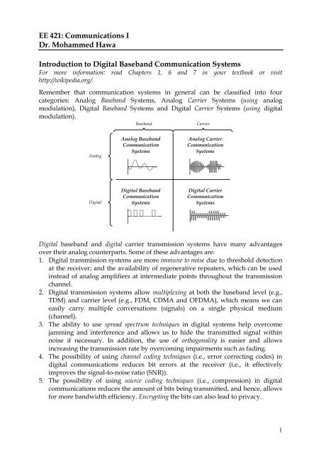
EE 421: Communications IDr. Mohammed HawaIntroduction to Digital Baseband Communication SystemsFor more information: read Chapters 1, 6 and 7 in your textbook or visithttp://wikipedia.org/.Remember that communication systems in general can be classified into fourcategories: Analog Baseband Systems, Analog Carrier Systems (using analogmodulation), Digital Baseband Systems and Digital Carrier Systems (using digitalmodulation).BasebandCarrierAnalogAnalog BasebandCommunicationSystemsAnalog CarrierCommunicationSystemsDigitalDigital BasebandCommunicationSystemsDigital CarrierCommunicationSystemsDigital baseband and digital carrier transmission systems have many advantagesover their analog counterparts. Some of these advantages are:1. Digital transmission systems are more immune to noise due to threshold detectionat the receiver; and the availability of regenerative repeaters, which can be usedinstead of analog amplifiers at intermediate points throughout the transmissionchannel.2. Digital transmission systems allow multiplexing at both the baseband level (e.g.,TDM) and carrier level (e.g., FDM, CDMA and OFDMA), which means we caneasily carry multiple conversations (signals) on a single physical medium(channel).3. The ability to use spread spectrum techniques in digital systems help overcomejamming and interference and allows us to hide the transmitted signal withinnoise if necessary. In addition, the use of orthogonality is easier and allowsincreasing the transmission rate by overcoming impairments such as fading.4. The possibility of using channel coding techniques (i.e., error correcting codes) indigital communications reduces bit errors at the receiver (i.e., it effectivelyimproves the signal-to-noise ratio (SNR)).5. The possibility of using source coding techniques (i.e., compression) in digitalcommunications reduces the amount of bits being transmitted, and hence, allowsfor more bandwidth efficiency. Encrypting the bits can also lead to privacy.1

6. Digital communication is inherently more efficient than analog systems inexchanging SNR for bandwidth, and allows such exchange at both the basebandand carrier levels.7. Digital hardware implementation is flexible and permits the use ofmicroprocessors. Using microprocessors to perform digital signal processing (DSP)eliminates the need to build expensive and bulky discrete-component devices. Inaddition, the price of microprocessors continues to drop every day.8. Digital signal storage is relatively easy and inexpensive. Also the reproduction ofdigital messages can be extremely reliable without deterioration, unlike analogsignals.Actually, due to those important advantages most of communication systemsnowadays are digital, with analog communication playing a minor role (we still, forexample, listen to analog AM and FM radio).This article provides a very quick overview of some of the main concepts that arerelevant to digital baseband transmission. You will study more about this topic in theEE422 “Communications II” course. The main concepts to be emphasized here willbe the analog-to-digital conversion process and the line coding concept.Digitization (and Analog-to-Digital (A/D) Conversion):Signals that result from physical phenomena (such as voice or video) are almostalways analog baseband signals. Converting such analog baseband signals into digitalbaseband signals is not as simple as one might expect, especially when consideringmodern communication systems such as Digital TV, SDH, Ethernet, ADSL, etc. Tosummarize, we say digitization involves the following steps:1. Sampling (in which the signal becomes a sampled analog signal, also called adiscrete analog signal).2. Quantization (the signal becomes a quantized discrete signal, but not a digitalbaseband signal yet).3. Mapping (the signal becomes a stream of 1‟s and 0‟s). Mapping is sometimesconfusingly called encoding.4. Encoding and Pulse Shaping (after which the signal becomes a digital basebandsignal).These four steps are shown in Figure 2 below and are explained in the followingsubsections.AnalogBasebandSignalA/D1's & 0'sEncoding &Pulse ShapingDigitalBasebandSignalDigitalModulationDigitalCarrierSignalSampling Quantization MappingSourceEncodingChannelEncodingLineEncodingPulseShaping(Optional) (Optional) (Mandatory) (Mandatory)Figure 2. The Many Steps of Digitization.2

impulses, as shown in Figure 4 below 4 . We will explain in class the differencebetween practically-sampled signals, naturally-sampled signals, and ideally-sampledsignals.Samples Values Sampled Signal, m s (t)m ptT sSampling Time-m pT sFigure 4. Practical Sampling.II. Quantization:The next step in analog-to-digital conversion is Quantization, which limits the digitaldata to be sent. Quantization is the process in which each sample value isapproximated or “limited to” a relatively-small set of discrete quantization levels. Forexample, in uniform quantization if the amplitude of the signal m(t) lies in the range(-mp, mp), we can partition this continuous range into L discrete intervals, each oflength v = 2 mp /L, and the value of each sample is then approximated to only oneof these L levels.Notice that quantization can be done in several different ways. In one method thevalue of each sample can be “truncated” to the quantization level just below it. Thisis shown in Figure 5 below for L = 5 levels.Sample Values now Quantizedm pm(t)errorQuantization Error = m s(t) – m sq(t) = [0, v]-m pFigure 5.m sq(t)vtL = 5Levels,Rule =Truncate4 Typical IC-based ADC chips perform sampling, quantization and mapping all on the same chip.4

Notice that the quantization error (i.e., the difference between the original samplevalue and the quantized sample value) is limited to the range [0, v]. Thisquantization error is a deliberate error introduced by the transmitter to control thetransmitted bit rate. Notice, however, that this error can be controlled by reducingthe value of v, which can be achieved by increasing the number of quantizationlevels L as shown in Figure 6 below where L = 10 levels now.Sample Values now Quantizedm pm(t)errorvtL = 10Levels,Rule =TruncateQuantization Error = m s(t) – m sq(t) = [0, v]-m pm sq(t)Figure 6.Another valid method of quantization is where samples are “rounded off” to thenearest quantization level either below it or above it. This is shown in Figure 7below. Notice that in this method the quantization error is now limited to [-v/2,v/2].errorSample Values now Quantizedm pm(t)vtL = 10Levels,Rule =Approx.Quantization Error = m s(t) – m sq(t) = [-v/2, v/2]-m pm sq(t)Figure 7.The number of quantization levels L is an important parameter in digital systemsbecause it decides (see next section) how many bits will be used to represent thevalue of each sample. For example, if L = 256, the value of each sample can be in oneof 256 possibilities, which means that each sample must be mapped (encoded) into 8bits. This is because 8 binary bits can be in 2 8 = 256 possible states (00000000,00000001, 00000010, 00000011, . . ., 11111111). For L = 65,536, we need 16 bits toencode each sample value.5

In voice telephony, for example, the number of quantization levels is chosen to beL = 2 8 = 256 since intelligibility (rather than high fidelity) is required, while forcompact disc (CD) audio, the number of quantization levels is L = 2 16 = 65,536possible values per sample. Of course, the bigger value of L means a smallerquantization error range v, and thus better quality.We will discuss in class how quantization can be visualized as a noise signal. We willalso explain how adaptive quantization can improve the signal-to-quantization-noiseratio (SQNR).III. Mapping:After the analog signal is discretized in time (i.e., sampled) and value (i.e.,quantized), it is converted into a binary bit stream using a process called mapping, inwhich each of the quantized sample values (e.g., 6V, 10V, etc) is mapped to acorresponding binary code (e.g., 0110, 1010, etc). The result is a stream of 1‟s and 0‟s.Notice that each sample is represented by n = log2 (L) bits, and hence the bit time T0is given by T0 = Ts / log2 (L), where Ts is the sample period. For example, if L = 256,we have T 0 = T s 8 (see Figure 8 below).The total number of bits generated in one second is called the data bit rate f0 = 1 / T0measured in bits/s (or bps) and is given by:f0 [bps] = fs [samples/s] × log2 (L) [bits/sample]m sq (t)T stT s0 1 1 0 0 1 0 0T 01 0 1 0 1 1 0 0T 0m digital (t)T s = log 2 (L)×T 0T s = log 2 (L)×T 0Figure 8. The Sampled Signal being Mapped into 1's and 0's.6

IV. Encoding:Now that we have a bit stream of 1‟s and 0‟s, those bits are first manipulated into anew (and better) sequence of 1‟s and 0‟s, and then converted into voltagesappropriate for transmission on a physical channel. This manipulation andconversion is collectively called encoding. Encoding schemes are usually dividedinto: source encoding, channel encoding and line encoding (see Figure 2).A. Source coding: Source coding refers to the process of compressing data. This istypically done by replacing long binary codewords that occur frequently by shorterones, and those that occur less frequently by longer codes. For example, a 4-bitsequence “0110” occurring frequently can be mapped into the shorter 2-bit sequence“01”, while another 4-bit sequence “1011” occurring less frequently can be mappedto the longer 6-bit sequence “111001”. This makes sure that sequences that occurmore often in the bit stream are the shorter ones.In information theory, Shannon's noiseless coding theorem places an upper andlower bounds on the expected compression ratio. Examples of source codescurrently in use are: Shannon codes, Huffman codes, run-length encoding (RLE),arithmetic coding, Lempel-Ziv coding, MPEG-2 and MPEG-4 video coding 5 , LinearPrediction Coding (LPC) and Code-Excited Linear Prediction (CELP) coding, etc.B. Channel coding: Channel coding refers to error correcting codes. The mostobvious example of such codes is the simple parity bit system. Such codes are used toprotect data sent over the channel from corruption even in the presence of noise. Inother words, channel codes can improve the signal-to-noise ratio (SNR) of thereceived signal.The theory behind designing and analyzing channel codes is called Shannon’s noisychannel coding theorem. It puts an upper limit on the amount of information youcan send in a noisy channel using a perfect channel code. This is given by thefollowing equation:C = B ch × log 2 1 + SNRwhere C is the upper bound on the capacity of the channel (bit/s), Bch is thebandwidth of the channel (Hz) and SNR is the Signal-to-Noise ratio on the channel(unitless). Examples of channel codes currently in-use include: Hamming codes,Reed-Solomon codes, convolutional codes (usually decoded by an iterative Viterbidecoder), Turbo codes, etc.C. Line coding: Line coding refers to the process of representing the final bit stream(1‟s and 0‟s) in the form of voltage or current variations optimally tuned for thespecific properties of the physical channel being used.The selection of a proper line code can help in so many ways: (a) One possibility is toaid in clock recovery at the receiver. A clock signal is recovered by observingtransitions in the received bit sequence, and if enough transitions exist, a goodrecovery of the clock is guaranteed, and the line code is said to be self-clocking. Self-5 MPEG is short for Moving Picture Experts Group.7

clocking is important in digital systems as all digital receivers require the existenceof the clock to function properly (this is similar to the synchronous detection processin DSB-SC demodulators).(b) Another advantage is to the ability to control the DC component in the resultingline code. This is important because most long-distance communication channelscannot transport a DC component 6 , and hence, most line codes try to eliminate theDC component before being transmitted on the channel. Such codes are called zero-DC or DC equalized.Other advantages of proper line coding include the (c) possibility of transmitting at ahigher data bit rate while requiring smaller bandwidth for the resulting basebandsignal, (d) the possibility of increasing the average power of the baseband signalcompared to noise (i.e., improving SNR), and (e) reducing the amount of power atlow-frequency components of the spectrum, which is important in telephone lineapplications, where the channel exhibits heavy attenuation below 300 Hz.Some types of line encoding in common-use nowadays are unipolar, polar, bipolar,Manchester, MLT-3 and Duobinary encoding. These codes are explained here:1. Unipolar (Unipolar NRZ and Unipolar RZ):Unipolar is the simplest line coding scheme possible, but the least used in practicedue to its many disadvantages. Unipolar coding uses a positive rectangular pulsep(t) to represent binary 1, and the absence of a pulse (i.e., zero voltage) to represent abinary 0.Two possibilities for the pulse p(t) exist 7 : Non-Return-to-Zero (NRZ) rectangularpulse and Return-to-Zero (RZ) rectangular pulse. The difference between UnipolarNRZ and Unipolar RZ codes is that the rectangular pulse in NRZ stays at a positivevalue (e.g., +5V) for the full duration of the logic 1 bit, while the pule in RZ dropsfrom +5V to 0V in the middle of the bit time. The figure below shows the differencebetween Unipolar NRZ and Unipolar RZ for the example bit stream 1110110001001.ClockData 1 1 1 0 1 1 0 0 0 1 0 0 1Code0T 0Bit timeT sSampling time (assuming 8 bits per sample)Unipolar NRZ Code6 DC-values create excessive heat generation in the channel, they cause baseline drift and also do notfit systems that carry an additional small direct current to power intermediate amplifiers (an exampleis telephone networks).7 Actually there are so many possibilities for the pulse shape p(t); not just a rectangular NRZ orrectangular RZ pulses. Changing p(t) waveform is called Pulse Shaping and affects the characteristicsof the line code as will be explained later.8

ClockData 1 1 1 0 1 1 0 0 0 1 0 0 1Code0T 0Bit timeUnipolar RZ CodeAn advantage of unipolar NRZ is that it is compatible with TTL logic. However, adrawback of unipolar (RZ and NRZ) is that its average value (i.e., DC value) is notzero (see the impulse at zero frequency in the corresponding power spectral density(PSD) of this line code shown in the diagram below). As we explained earlier, a DCvalueis not desired in long-distance communication systems. Another disadvantageof such unipolar (RZ and NRZ) signaling is that it does not include clock informationespecially when the bit stream consists of a long sequence of 0‟s.The disadvantage of unipolar RZ compared to unipolar NRZ is that each rectangularpulse in RZ is only half the length of the NRZ pulse. This means that unipolar RZrequires twice the bandwidth of the NRZ code. This can be seen from the PSD ofboth signals shown below 8 .S m (w)Unipolar NRZS m (w)Unipolar RZw-8pf 0 -6pf 0 -4pf 0 -2pf 0 0 2pf 0 4pf 0 6pf 0 8pf 0 -8pf 0 -6pf 0 -4pf 0 -2pf 0 0 2pf 0 4pf 0 6pf 0 8pf 0-4f 0 -3f 0 -2f 0 -f 0 0 f 0 2f 0 3f 0 4f 0 -4f 0 -3f 0 -2f 0 -f 0 0 f 0 2f 0 3f 0 4f 0ffw2. Polar (Polar NRZ and Polar RZ):In Polar NRZ line coding a binary 1 is represented by a pulse p(t) (e.g., +5V) and abinary 0 is represented by the negative of this pulse -p(t) (e.g., -5V). Polar (NRZ andRZ) signals are shown in the diagram below.Using the assumption that in a regular bit stream a logic 0 is just as likely as a logic 1,polar line codes (whether RZ or NRZ) have the advantage that the resulting DCcomponentis very close to zero.8 The above spectra were calculated based on the assumption that logic 1‟s and logic 0‟s are equally likely in thetransmitted bit sequence. This is a simplifying assumption that we use throughout this article.9

Polar NRZ CodePolar RZ CodeIn addition, the rms value of polar signals is bigger than unipolar signals, whichmeans that polar signals have more power than unipolar signals 9 , and hence havebetter SNR at the receiver. Actually, polar NRZ signals have more power comparedto polar RZ signals.The drawback of polar NRZ, however, is that it lacks clock information especiallywhen a long sequence of 0‟s or 1‟s is transmitted. This problem does not exist inpolar RZ signals, since the signal drops to zero in the middle of each pulse period.The power spectral densities (PSD) of both polar NRZ and polar RZ are shownbelow.S m (w)Polar NRZPolar RZ-8pf 0 -4pf 0 -2pf 0 0 2pf 0 4pf 0 6pf 0 8pf 0w-6pf 0f-4f 0 -3f 0 -2f 0 -f 0 0 f 0 2f 0 3f 0 4f 0Signals transmitted on a computer motherboard often use Polar NRZ code. Anotheruseful application of this encoding is in Fiber-based Gigabit Ethernet (1000BASE-SXand 1000BASE-LX).9 2Remember that the average power in a signal is the square of its rms value (P x = x rms ).10

A variant of Polar NRZ is Non-Return-to-Zero-Level (NRZ-L) in which the 1‟s and0‟s are represented by -p(t) and p(t), respectively. This is Polar NRZ using negativelogic. An example where NRZ-L is used is the legacy RS-232 serial portcommunication.NRZ-L Code3. Non-Return-to-Zero, Inverted (NRZI):NRZI is a variant of Polar NRZ. In NRZI there are two possible pulses, p(t) and -p(t).A transition from one pulse to the other happens if the bit being transmitted is alogic 1, and no transition happens if the bit being transmitted is a logic 0.NRZI Code 10This is the code used on compact discs (CD), USB ports, and on fiber-based FastEthernet at 100-Mbit/s (100Base-FX).NRZI can achieve synchronization between the transmitter and receiver, if we makesure that there are enough umber of 1‟s in the transmitted bit stream.4. Bipolar encoding (also called Alternate Mark Inversion (AMI)):Bipolar (or AMI) is a three-level system that uses p(t), -p(t), and the absence of pulses(e.g. +5V, -5V, 0V) to represent logical values. A logic 0 is represented with an absentpulse, and a logic 1 by either a positive or negative pulse. The direction of the pulseis opposite of the pulse sent for the previous logic 1 (mark) (see the Figure below).10 NRZI is always polar not unipolar.11

Bipolar (AMI) CodeThe alternating code in bipolar encoding prevents the build-up of a DC voltage inthe cable. You can also observe the absence of low frequencies (including the DCcomponent) from the PSD for AMI shown below.S m (w)Duobinary Line Code BandwidthBipolar NRZ (AMI) Unipolar NRZ f 0Unipolar RZ 2 f 0Polar NRZPolar NRZ f 0Polar RZ 2 f 0Polar RZBipolar NRZ f 0Duobinary f 0 / 20 2pf 04pf 00f 02f 0wfAMI coding was used extensively in first-generation digital telephony PCMnetworks. AMI suffers the drawback that a long run of 0's produces no transitions inthe data stream, and a loss of synchronization is possible. This was solved intelephony by adopting improved variants of AMI encoding to ensure regulartransitions in the baseband signal even for long runs of 0‟s. The Binary-with-8-Zero-Substitution (B8ZS) is the line coding scheme that was adopted for North AmericaT1 system, while High-Density Bipolar 3-Levels (HDB3) was the line codingscheme used in the European E1 system.This is not part of the exam material …Note: A very similar encoding scheme to AMI, with the logical positions reversed, isalso used and is often referred to as pseudoternary encoding. This encoding isessentially identical to AMI, with marks (1‟s) being zero voltage and spaces (0‟s)alternating between positive and negative pulses.Note: Coded Mark Inversion (CMI) is another variation of AMI, where 0 bits arerepresented by a transition in the middle of the bit time instead of zero voltage.12

5. Duobinary:In a duobinary line code a 0 bit is represented by a zero-level electric voltage; a 1 bitis represented by a p(t) if the quantity of 0 bits since the last 1 bit is even, and by -p(t)if the quantity of 0 bits since the last 1 bit is odd. An illustration of the duobinary linecode is shown below.ClockData 1 1 1 0 1 1 0 0 0 1 0 0 1Code0Duobinary CodeFor a bit rate of f0, duobinary line code requires f0/2 bandwidth, which is theminimum possible (theoretical) bandwidth for any digital baseband signal (calledNyquist bandwidth). In addition, the duobinary line code permits the detection ofsome transmission errors without the addition of error-checking bits. However,duobinary line codes have significant low frequency components as seen by the PSDshown earlier. The differential version of the duobinary line code is common in the20 Gbit/s and 40 Gbit/s uncompensated optical fiber transmission systems.It is important, however, that you do not confuse a duobinary line code (explainedabove) with something completely different called a duobinary pulse (shown below).This pulse (which you are going to study in the “Communications II” course) iscommonly used in controlled inter-symbol interference (ISI) scenarios. Confusingly,duobinary signaling refers to using the duobinary pulse with a polar line coding rule(not a duobinary line coding rule).p(t) = Duobinary Pulse1 V-3T 0-2T 0-T 00T 02T 03T 0t6. Multi-Level Transmission 3-Levels (MLT-3):MLT-3 encoding is used mainly in 100BASE-TX Fast Ethernet, which is the mostcommon type of Ethernet nowadays. MLT-3 cycles through the states -p(t), 0, p(t), 0,-p(t), 0, p(t), 0, ... etc. It moves to the next state to transmit a 1 bit, and stays in thesame state to transmit a 0 bit.MLT-3 has many advantages including emitting less electromagnetic interference,requiring less bandwidth than unipolar, polar, and bipolar (AMI) signals operatingat the same data bit rate. The PSD of MLT-3 code is shown in Figure 22.13

MLT-3 Code7. Manchester:There are two opposing conventions for the representation of Manchester codes:The first convention of these was first published by G. E. Thomas in 1949 and isfollowed by numerous authors (e.g., Andrew S. Tanenbaum). It specifies that for a 0bit the signal levels will be Low-High with a low level in the first half of the bitperiod, and a high level in the second half (see figure below). For a 1 bit the signallevels will be High-Low.The second convention is also followed by numerous authors (e.g., Stallings) as wellas by IEEE 802.4 and IEEE 802.3 (Ethernet 10 Mbps 10Base-T) standards. It statesthat a logic 0 is represented by a High-Low signal sequence and a logic 1 isrepresented by a Low-High signal sequence.If a Manchester encoded signal gets inverted somewhere along the communicationpath, it transforms from one variant to another. In this article, we will adopt the firstconvention (see figure below).Manchester Code 11In a Manchester code each bit of data is signified by at least one transition.Manchester encoding is therefore considered to be self-clocking, allowing anaccurate clock recovery from the data stream. In addition, the DC component of theencoded signal is zero.11 Manchester is always polar not unipolar.14

Although transitions allow the signal to be self-clocking, it carries significantoverhead as there is a need for essentially twice the bandwidth of a simple PolarNRZ or NRZI encoding (see the PSD below). This is the main disadvantage of theManchester code.S m (w)MLT-3Polar NRZManchesterPolar RZLine Code BandwidthPolar NRZ f 0Polar RZ 2 f 0MLT-3 0.9 f 0Manchester 2 f 00 2pf 04pf 00f 02f 0wfFigure 22.This is not part of the exam material …Differential Manchester encodingIn Differential Manchester encoding a 1 bit is indicated by making the first half of thesignal equal to the last half of the previous bit‟s signal i.e. no transition at the start ofthe bit-time. A 0 bit is indicated by making the first half of the signal opposite to thelast half of the previous bit's signal i.e. a zero bit is indicated by a transition at thebeginning of the bit-time.Differential Manchester CodeBecause only the presence of a transition is important, differential schemes will workexactly the same if the signal is inverted (wires swapped).In the middle of the bit-time there is always a transition, whether from high to low,or low to high, which provides a clock signal to the receiver.Differential Manchester is specified in the IEEE 802.5 standard for IBM Token RingLANs, and is used for many other applications, including magnetic and opticalstorage.15

8. M-ary CodingAll the line coding schemes discussed above are called binary codes, since thenumber of bits per second is identical to the number of symbols per second (calledbaud rate). We say that for binary signaling:f0, data bit rate [in units of bit/s] = fsymb, symbol rate [in units of baud]Notice that a symbol is defined as a waveform pattern that the line code has for acertain period of time before switching to another waveform pattern (i.e., anothersymbol).In M-ary signaling, on the other hand, a cluster of bits is grouped to represent onesymbol. For example, in the 4-ary (also called Quaternary) case, two bits are groupedinto one symbol. The two bits can be in one of 4 possible states, which means that thesymbol can take M=4 different symbols. The following table shows a possiblemapping of two bit values to four symbols of a Quaternary signal. Thecorresponding line code for this Quaternary signal representing the bit stream1110110001001 is shown next.Bits Symbol00 -5 V01 -10 V10 5 V11 10 VM=4levelsClockData10 V1 1 1 0 1 1 0 0 0 1 0 0 15 VCode-5 V0-10 VT 0 Bit TimeT symb Symbol TimeT sSampling Time (assuming 8 bits per sample)Quaternary CodeNotice that a symbol time Tsymb is now twice the bit time T0. This means that there arehalf as much symbol transitions as there are bit transitions. We can say that:symbol rate [in units of baud] = (½) × data bit rate [in units of bit/s]For a general M-ary line coding scheme, we have:symbol rate [in units of baud] = (1/log2 (M)) × data bit rate [in units of bit/s]16

where M is the number of levels (possibilities) for a symbol. Such a drop in transitionrate in the resulting signal will reduce the bandwidth of the signal by a factor oflog2 (M), because the bandwidth of digital signal is actually dependent on its baudrate fsymb not its bit rate f0.Remember: An M-ary signal is a baseband signal that has a bandwidth equal to itsbaud rate (fsymb). The PSD of the M-ary signal is shown below.S m (w)M-ary-4pf symb -2pf symb02pf symb 4pf symbf-2f symb 0-f symbf symb2f symbwV. Pulse Shaping:In explaining the above line codes, we limited ourselves to pulses p(t) shaped aseither rectangular NRZ or rectangular RZ pulses. It is essential that you understandthat these two are not the only choices you have; instead a variety of pulse shapesp(t) can be used without compromising the information transfer process. In thissection, we will discuss two possibilities: the triangular pulse and the raised cosinepulse. The Figure below shows the bit stream 1110110001001 represented using apolar line code combined with a triangular pulse shape.ClockData 1 1 1 0 1 1 0 0 0 1 0 0 1Code0Figure 25.You might be wondering at this point about the advantages of choosing a pulseshape different than the simple and familiar rectangular pulse? Well, there is anumber of advantages for doing so, the main of which is being able to control theshape of the power spectral density PSD (and hence the bandwidth) of the resultingdigital baseband signal.To understand this, recall that the line code you chose earlier (unipolar, polar,bipolar, etc) has affected the bandwidth of the corresponding code. However, thePSD shape always looked like a sinc 2 () function. The reason this was the case is thatthe Fourier transform of a rectangular pulse has the sinc() shape and because thePSD is the square of the Fourier transform, the PSD looked like a sinc 2 () function (seeFigure 27).17

You also recall that using a RZ rectangular pulse instead of a NRZ rectangular pulseresulted in expanding the bandwidth by a factor of 2. This is an immediate result ofthe “Time compression, Frequency expansion” property of the Fourier transform,and is also illustrated in Figure 27.The question that arises now is this: If we pick a data stream encoded using aparticular line code (say polar encoding), can we control its bandwidth by changingthe pulse shape p(t) while still keeping the polar line code rule? The answer to thisquestion is YES; picking the right pulse shape can result in smaller bandwidthcompared to the bandwidth of the rectangular pulse which is, strictly-speaking,infinity (because the sinc() function extends from minus infinity to positive infinity).If we choose a smoother pulse (compared to the rectangular pulse), the highfrequencies in the resulting PSD of the data stream are eliminated. For example, ifwe pick a triangular pulse instead of a rectangular pulse (see Figure 27) the highfrequency components are heavily reduced. (This is more apparent if you look at thespectrum using a log scale). Remember that the Fourier transform of a triangularpulse is sinc 2 () and, hence, the PSD has the shape of sinc 4 () function.Reducing high frequency components in the PSD is important so that the signal canpass through band-limited channels without too much linear distortion. Suchdistortion usually creates what is called inter-symbol interference (ISI) in digitalsystems, where one bit value overlaps with (and corrupts) the adjacent bits.Using smoother pulses (and hence reducing their high frequency content) can betaken to the extreme if we pick a pulse that is not limited in time. In other words, thepulse spells outside the bit time (T0). This will limit its Fourier transform (because anexpansion in the time-domain results in compression in the frequency-domain).One popular example used in many practical systems is the raised-cosine pulse. This isa pulse that looks similar to (but decays much quicker than) a sinc(t) function and has aFourier transform similar to a raised cosine shape in the frequency domain. Thispulse and its corresponding Fourier transform are shown below. The raised-cosinepulse shape changes with a parameter called the roll-off factor . The Figure belowshows a = 0.5 raised-cosine pulse with the corresponding Fourier transform.1 Vp(t) = Raised Cosine PulseP(w)T 0 f 0/2-3T 0-2T 0-T 00T 02T 03T 0tw- 2pf 0 - pf 0 0pf 0 2pf 0f- f 0 - f 0/2 0 f 0/2f 0This type of pulse satisfies what is called the first Nyquist ISI criterion, which statesthat it is OK for the pulse shape not to be limited to the bit time (T0), so long as itdoes not introduce inter-symbol interference (ISI) in the transmitted pulse stream.18

P(w)S p(w)p(t)Fourier TransformPower SpectralDensityT 0Bit timet-8pf0-6pf0-4pf0-2pf0w0 -8pf0 -6pf0 -4pf0 -2pf0 0 2pf0 4pf02pf0 4pf0 6pf0 8pf06pf0w 8pf0S p(w) [Log Scale]-8pf0-6pf0-4pf0-2pf002pf04pf06pf0w 8pf0P(w)S p(w)p(t)Fourier TransformPower SpectralDensityT 0Bit timet-8pf0-6pf0-4pf0-2pf0w0 -8pf0 -6pf0 -4pf0 -2pf0 0 2pf0 4pf02pf0 4pf0 6pf0 8pf06pf0w 8pf0S p(w) [Log Scale]-8pf0-6pf0-4pf0-2pf002pf04pf06pf0w 8pf0P(w)S p(w)p(t)Fourier TransformPower SpectralDensityT 0Bit timet-8pf0 -6pf0 -4pf0 -2pf0w0 -8pf0 -6pf0 -4pf0 -2pf0 0 2pf0 4pf02pf0 4pf0 6pf0 8pf06pf0w 8pf0S p(w) [Log Scale]-8pf0 -6pf0 -4pf0 -2pf002pf04pf06pf0w 8pf0P(w)S p(w)p(t)Fourier TransformPower SpectralDensityT 0Bit timet-8pf0 -6pf0 -4pf0 -2pf00 w-8pf0 -6pf0 -4pf0 -2pf0 0 2pf0 4pf02pf0 4pf0 6pf0 8pf06pf0w 8pf0T 0S p(w) [Log Scale]Figure 27.-8pf0 -6pf0 -4pf0 -2pf002pf04pf06pf0w 8pf019

An example of using the raised-cosine pulse combined with polar line code is shownin Figure 28, where the binary sequence „1011011100‟ is transmitted. Notice that weuse p(t) for logic 1 and -p(t) for logic 0 (i.e., the polar line code). The dotted linesrepresent the raised-cosine pulses p(t) and -p(t) corresponding to individual bits,while the solid line represents the result of adding these pulses (i.e., the transmittedsignal on the channel). At the receiver side, sampling the received signal at exactlythe middle of the bit time will retrieve the original bit sequence as shown in theFigure.Our example used raised-cosine pulses with parameter = 0.5. In such case, thebandwidth of the resulting stream is given by the formula (1+) f0 / 2 = (1+0.5) f0 / 2= 0.75 f0, where f0 is the data rate. Hence, if f0 = 50 kbit/s, the resulting bandwidth =37.5 kHz. What would the bandwidth have been if you used a rectangular NRZpulse? How about a rectangular RZ pulse?ClockData 1 0 1 1 0 1 1 1 0 01 V0-1 VTXsignal1 V-1 V1 VRXsampling-1 VFigure 28.20