Integration - the Australian Mathematical Sciences Institute

More documents

Recommendations

Info

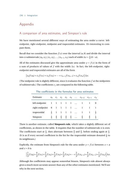
{34} • IntegrationAppendixA comparison of area estimates, and Simpson’s ruleWe have mentioned several different ways of estimating the area under a curve: leftendpoint,right-endpoint, midpoint and trapezoidal estimates. It’s interesting to comparethem.Recall that we consider the function f (x) over the interval [a,b] and divide the intervalinto n subintervals [x 0 , x 1 ],[x 1 , x 2 ],...,[x n−1 , x n ] each of width ∆x = 1 n(b − a).All of the estimates discussed give the approximate area under y = f (x) in the form ofa sum of products of values of f with the width ∆x. In fact, the left-endpoint, rightendpointand trapezoidal estimates are all of the form[c0 f (x 0 ) + c 1 f (x 1 ) + c 2 f (x 2 ) + ··· + c n−1 f (x n−1 ) + c n f (x n ) ] ∆x.(The midpoint rule is slightly different, since it evaluates the function f at the midpointsof subintervals.) The coefficients c j are compared in the following table.The coefficients in the formulas for area estimatesEstimate c 0 c 1 c 2 c 3 c 4 ... c n−2 c n−1 c nleft endpoint 1 1 1 1 1 ... 1 1 0right endpoint 0 1 1 1 1 ... 1 1 1trapezoidalSimpson121 1 1 1 ... 1 11343234323...23431213There is another estimate, called Simpson’s rule, which takes a slightly different set ofcoefficients, as shown in the table. It requires that the number of subintervals n is even.The coefficients start at 1 3 , then alternate between 4 3 and 2 3 , before ending again at 1 3 .(It is as if every second coefficient in the list for the trapezoidal estimate donated 1 6 toits neighbours.)Explicitly, the estimate from Simpson’s rule for the area under y = f (x) between x = aand x = b is[ 13 f (x 0)+ 4 3 f (x 1)+ 2 3 f (x 2)+ 4 3 f (x 3)+ 2 3 f (x 4)+···+ 2 3 f (x n−2)+ 4 3 f (x n−1)+ 1 3 f (x n)]∆x.Although the coefficients may appear somewhat bizarre, Simpson’s rule almost alwaysgives a much more accurate answer than any of the other estimates mentioned. We’ll seewhy in the next section.
A guide for teachers – Years 11 and 12 • {35}Exactness of area estimatesConsider some simple functions f (x) — constant, linear, quadratic — and see how thevarious estimates fare in approximating the integral ∫ baf (x) d x.First suppose f (x) is a constant function. In this case, we obtain an exactly correct answerfor the area under the graph from the left-endpoint, right-endpoint, midpoint ortrapezoidal estimate. The area under y = f (x) is itself a rectangle; breaking it up intorectangles or trapezia, we still have the exactly correct area. This is true regardless of thenumber of subintervals n: we could split [a,b] into just one subinterval, or a million; inall cases we obtain the exactly correct answer.yy0 abArea under a constant function.x0aArea under a linear function,correctly estimated by midpoint ortrapezoidal estimate.bxNext suppose f (x) is a (non-constant) linear function. In this case the left- and rightendpointestimates will definitely not give you the correct answer. However, the midpointand trapezoidal estimates will give you the exactly correct answer. The midpointestimate builds rectangles which have exactly the same amount of area above and belowthe line. And breaking the area under y = f (x) into trapezia gives the exactly correct area.Again this is true whatever number of subintervals we take.However, when f (x) is a quadratic function, in general none of the left-endpoint, rightendpoint,midpoint or trapezoidal estimates will give the correct area. Let’s consider thefunction f (x) = x 2 , and see how the midpoint and trapezoidal estimates fare. We’ll justtake one subinterval, n = 1, so ∆x = b − a.First, the midpoint estimate M is just( a + b) ( 1M = f ∆x =24 a2 + 1 2 ab + 1 4 b2) ( )b − a .Next, the trapezoidal estimate T (again with only one subinterval) is( 1T =2 f (a) + 1 ) ( 12 f (b) ∆x =2 a2 + 1 2 b2) ( )b − a .
Page 1 and 2: 1Supporting Australian Mathematics
Page 3 and 4: Assumed knowledge . . . . . . . . .
Page 5 and 6: A guide for teachers - Years 11 and
Page 33: A guide for teachers - Years 11 and

Integration - the Australian Mathematical Sciences Institute

You also want an ePaper? Increase the reach of your titles

Delete template?

Save as template?