Numerical Solutions of Linear Systems of Equations

EE 216 Class NotesGAUSS ELIMINATIONThe operations in the Gauss elimination are called elementary operations.Elementary operations for equations are:(I)(II)(III)Interchange of two equations.Multiplication of an equation by a nonzero constant.Addition of a constant multiple of one equation to another equation.Let us consider the set of linearly independent equations.2x - 4y + 5z = 36 … … (1)- 3x + 5y + 7z = 7 … … (2)5x + 3y - 8z = - 31 … … (3)Augmented matrix for the set is:⎛⎜⎜⎜⎝2− 35− 45357− 836 ⎞7− 31⎟⎟⎟⎠Step 1Eliminate x from the 2 nd and 3 rd equation.3R ′ +22→ R1R25R ′ → − +23R1R3Pages 3 of 21

EE 216 Class NotesFrom Row 3, 176z = -704Therefore, z = - 704/176 = - 4From Row 2, 19y – 2z = 103or, 19y – 2 (- 4) = 103or, y = 5From Row 1, - 4x + 3y + 2z = -5or, - 4x + 3 (5) + 2 (- 4) = -5or, x = 3Elementary operations for equations and matrices are:(I)(II)(III)Interchange of two equations.Multiplication of an equation by a nonzero constant.Addition of a constant multiple of one equation to another equation.When would you interchange two equations (rows)?Let us consider the following set of equations.3y + 2z = 16 … … (1)4x + 2y - 3z = - 10 … … (2)3x + 4y + z = 9 … … (3)The corresponding augmented matrix is:⎛04⎜⎜⎜⎝33242− 3116⎞− 109⎟⎟⎟⎠Pages 6 of 21

EE 216 Class NotesEqn. (1) (Row 1) cannot be used to eliminate x from Eqns. (2) and (3) (Rows 2 and 3).Interchange Row 1 with Row 2.The augmented matrix becomes:⎛40⎜⎜⎜⎝3234− 321− 10⎞169⎟⎟⎟⎠Now follow the steps mentioned earlier to solve for the unknowns.The solution is:x = - 3y = 4z = 2Let us consider the following set of linear equations.2x 1 – 4x 2 + 5x 3 = 36 … … (1)- 3x 1 + 5x 2 + 7x 3 = 7 … … (2)5x 1 + 3x 2 – 8x 3 = - 31 … … (3)Gauss elimination suggests doing elementary row operations from top to bottom. Aslightly modified form, known as Gauss-Jordan elimination suggests doing elementaryrow operations from bottom to top as well.Pages 7 of 21

EE 216 Class NotesPages 8 of 21⎥⎥⎥⎥⎥⎥⎦⎤⎢⎢⎢⎢⎢⎢⎣⎡−−−−317368357535423132122523RRRRRR +→ −′+→′⎥⎥⎥⎥⎥⎥⎦⎤⎢⎢⎢⎢⎢⎢⎣⎡−−−- 12161362411302291054233131 RR →′⎥⎥⎥⎥⎥⎥⎦⎤⎢⎢⎢⎢⎢⎢⎣⎡−−−- 121/13613626411022910542323 RRR +→′⎥⎥⎥⎥⎥⎥⎦⎤⎢⎢⎢⎢⎢⎢⎣⎡−−672/1361361316800229105423316813 RR →′⎥⎥⎥⎥⎥⎥⎦⎤⎢⎢⎢⎢⎢⎢⎣⎡−−46136100229105423223112295 RRRRRR−→′−→′⎥⎥⎥⎥⎥⎥⎦⎤⎢⎢⎢⎢⎢⎢⎣⎡−−4316100010042

EE 216 Class NoteswhereD =aaa112131aaa122232aaa132333D =1bbb123aaa122232aaa132333D =2aaa112131bbb123aaa132333D =3aaa112131aaa122232bbb123Let us consider the following set of linear equations.2x 1 – 4x 2 + 5x 3 = 36 … … (1)- 3x 1 + 5x 2 + 7x 3 = 7 … … (2)5x 1 + 3x 2 – 8x 3 = - 31 … … (3)[A][x] = [B]where[ A]=⎡−⎢⎢⎢⎣235− 4535⎤7− 8⎥⎥⎥⎦⎡ x⎢⎢⎢⎣x1⎤⎥⎥⎥⎦[ x]= x and [ B]23=⎡ 36⎤7⎢⎢⎢⎣−31⎥⎥⎥⎦Pages 11 of 21

EE 216 Class NotesD =2− 35− 45357− 8= −33636 − 4 5D1 = 7 5 7 = − 672− 31 3 − 82 36 5D2= − 3 7 7 = 10085 − 31 − 82 − 4 36D3 = − 3 5 7 = −13445 3 − 31x− 672− 33611= == DD2xx1008− 33622= = −= DD= DD− 1344=− 33633=43Pages 12 of 21

EE 216 Class NotesSolve the following set of linear equations.x 1 + x 2 + x 3 = 2 … … (1)2x 1 + 5x 2 + 3x 3 = 11 … … (2)- x 1 + 2x 2 + x 3 = 3 … … (3)Solution by Matrix InversionConsider the following set of linear equations.a =11x1+ a12x2+ a13x3b1a =21x1+ a22x2+ a23x3b2a =31x1+ a32x2+ a33x3b3… … (1)… … (2)… … (3)The system of equations above can be written in matrix form as:⎡aa⎢⎢⎢⎣a112131aaa122232aaa132333⎤ ⎡ xx⎥⎥⎥⎦ ⎢⎢⎢⎣x123⎤⎥⎥⎥⎦=⎡bb⎢⎢⎢⎣b123⎤⎥⎥⎥⎦[A][x] = [B]where[ A]=⎡aa⎢⎢⎢⎣a112131aaa122232aaa132333⎤⎥⎥⎥⎦Pages 13 of 21

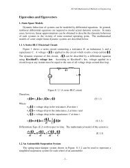
EE 216 Class Notes⎡ x⎢⎢⎢⎣x1⎤⎥⎥⎥⎦[ x] = x and [ B]23=⎡bb⎢⎢⎢⎣b123⎤⎥⎥⎥⎦If D ≠ 0 , then the system has a unique solution.[x] = [A] -1 [B]A Traffic Light AssemblyzCDA6 m4 mhB3 mx4 m3 m4 m6 m4 m3 myFigure 1.1 A traffic light assemblyThe mass of the traffic light assembly is 20 kg and h = 3.5 m. For equilibrium,the forces acting on the light assembly in all three directions (x, y and z) should equal tozero.∑ x∑ y∑ zF = 0 , F = 0 and F = 0Pages 14 of 21

EE 216 Class NotesBased on the above, a set of equations in terms of the three unknown forces canbe written as:0 .5970F− 0.8381F+ 0.7960F= 0AB0 .7960F− 0.4191F− 0.5970F= 0AB0 .0995F0.3492F+ 0.0995F= 196.2ACACAB+ACADADAD… … (1)… … (2)… … (3)[A][F] = [B]where[ A ]⎡0.5970= 0.7960⎢⎢⎢⎣0.0995− 0.8381− 0.41910.34920.7960⎤− 0.59700.0995⎥⎥⎥⎦⎡F⎢⎢⎢⎣FAB⎤⎥⎥⎥⎦[ F ] = F and [ B]ACAD[ F ] = [A]−1 [ B]=⎡ 0⎤0⎢⎢⎢⎣196.2⎥⎥⎥⎦[ ]−A 1=⎡−⎢⎢⎢⎣0.35470.29480.67990.7685− 0.0421− 0.62071.7737⎤2.10560.8867⎥⎥⎥⎦[ F ]=⎡−⎢⎢⎢⎣0.35470.29480.67990.7685− 0.0421− 0.62071.7737⎤⎡ 0⎤2.1056 00.8867⎥⎥⎥⎦ ⎢⎢⎢⎣196.2⎥⎥⎥⎦Pages 15 of 21

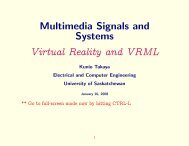
EE 216 Class Notes[ F ]⎡F= F⎢⎢⎢⎣FABACAD⎤ ⎡347.997⎤= 413.126⎥⎥⎥⎦ ⎢⎢⎢⎣173.978⎥⎥⎥⎦Therefore, F AB = 347.997 N, F AC = 413.126 N and F AD = 173.978 NAn Electrical CircuitBased on the principles of voltage drops (Kirchoff’s voltage law) and current flow(Kirchoff’s current law), the following equations can be written in terms of the unknowncurrent flow.20 ohms 15 ohmsI 1I 280 V+-12 ohmsI 3+-120 VFigure 2.1 An electrical circuit20I 1+ 12I3= 80 … … (2.1)15I 2+ 12I3= 120 … … (2.2)I + I − I 0 … … (2.3)1 2 3=The set of equations can be solved by substitution method in the following manner.Pages 16 of 21

EE 216 Class Notes[A][C] = [B]where[ A ]=⎡200⎢⎢⎢⎣ 1015112⎤12− 1⎥⎥⎥⎦⎡I⎢⎢⎢⎣I1⎤⎥⎥⎥⎦[ C ] = I and [ B][ C ] = [A]−1 [ B]23⎡ 80⎤= 120⎢⎢⎢⎣ 0⎥⎥⎥⎦[ ]−A 1[ C ]==⎡−⎢⎢⎢⎣⎡−⎢⎢⎢⎣0.03750.01670.02080.03750.01670.0208− 0.01670.04440.0278− 0.01670.04440.02780.2500⎤0.3333− 0.4167⎥⎥⎥⎦0.2500⎤⎡ 80⎤0.3333 120− 0.4167⎥⎥⎥⎦ ⎢⎢⎢⎣ 0⎥⎥⎥⎦[ C]=⎡II⎢⎢⎢⎣I123⎤⎥⎥⎥⎦=⎡1⎤4⎢⎢⎢⎣5⎥⎥⎥⎦Therefore, I 1 = 1 A, I 2 = 4 A and I 3 = 5 A.Pages 17 of 21

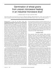
EE 216 Class NotesFlow Through a Piping Networkd = 0.5 mL = 150 md = 0.5 mL = 300 mBd = 0.5 mL = 300 mD0.09 m 3 /s0.03 m 3 /sAd = 0.75 mL = 300 md = 0.75 mL = 300 md = 0.5 mL = 150 mCd = 0.5 mL = 300 m0.06 m 3 /sd = 0.75 mL = 300 mFigure 3.1 A piping networkA set of equations can be written based on the following principles:1. At each junction, flow in = flow out.2. Kinetic energy and potential energy of the fluid makes the fluid movethrough the piping network.3. For a given fluid flow, the velocity increases and the pressure decreaseswhen the pipe diameter is decreased.4. Frictional loss is directly proportional to the length of the pipe and theviscosity of the fluid and inversely proportional to the diameter of the pipe.A set of equations as functions of the five unknown flow rates can be written as:Q Q = 0.03 … … (3.1)AB+ AC− Q + Q + Q = 0.06 … … (3.2)ACABCBCD+ QCB− QBD= 0Q … … (3.3)29 .9 − 29.9Q− 3.9Q= 0Q … … (3.4)ABACCB3 .9 − 7.9Q+ 19.9Q= 0Q … … (3.5)CBCDBDPages 18 of 21

EE 216 Class NotesIt should be noted that Eqns. (3.1) – (3.3) have been derived based on the principle ofconservation of mass. Eqns. (3.4) and (3.5) have been derived based on the principle ofpressure drop along pipe sections.The set of equations can be solved by substitution method in the following manner.[A][Q] = [B]where[ A ]=⎡ 10129.9⎢⎢⎢⎢⎢⎢⎣ 01− 10− 29.90011− 3.93.90100− 7.90⎤0− 1019.9⎥⎥⎥⎥⎥⎥⎦⎡QQQ⎢⎢⎢⎢⎢⎢⎣QABAC⎤⎥⎥⎥⎥⎥⎥⎦[ Q] = Q and [ B]CBCDBD[ Q]= [A]−1 [ B]⎡0.03⎤0.06= 00⎢⎢⎢⎢⎢⎢⎣ 0⎥⎥⎥⎥⎥⎥⎦Pages 19 of 21

EE 216 Class Notes[ ]−A 1⎡ 0.48830.5117= − 0.1790.6907⎢⎢⎢⎢⎢⎢⎣ 0.30930.0154− 0.01540.23570.74890.25110.0387− 0.03870.5938− 0.6325− 0.36750.0158− 0.0158− 0.0139− 0.00190.00190.0019⎤− 0.00190.0298− 0.03180.0318⎥⎥⎥⎥⎥⎥⎦[ Q]=⎡ 0.48830.5117− 0.1790.6907⎢⎢⎢⎢⎢⎢⎣ 0.30930.0154− 0.01540.23570.74890.25110.0387− 0.03870.5938− 0.6325− 0.36750.0158− 0.0158− 0.0139− 0.00190.00190.0019⎤⎡0.03⎤− 0.0019 0.060.0298 0− 0.0318 00.0318⎥⎥⎥⎥⎥⎥⎦ ⎢⎢⎢⎢⎢⎢⎣ 0⎥⎥⎥⎥⎥⎥⎦[ Q]⎡QQ= QQ⎢⎢⎢⎢⎢⎢⎣QABACCBCDBD⎤ ⎡0.0156⎤0.0144= 0.00870.0657⎥⎥⎥⎥⎥⎥⎦ ⎢⎢⎢⎢⎢⎢⎣0.0243⎥⎥⎥⎥⎥⎥⎦Therefore,Q AB = 0.0156 m 3 /s, Q AC = 0.0144 m 3 /sQ CB = 0.0087 m 3 /s, Q CD = 0.0657 m 3 /sQ BD = 0.0243 m 3 /sPages 20 of 21

EE 216 Class NotesSolve the following set of linear equations.x 1 + x 2 + x 3 = 2 … … (1)2x 1 + 5x 2 + 3x 3 = 11 … … (2)- x 1 + 2x 2 + x 3 = 3 … … (3)Exercise SetsSolve the following sets of linear equations by Gaussian elimination, Gauss-Jordanelimination, Cramer’s rule and matrix inversion.(1)4x − x + x = 8(2)2x1112+ 5xx + 2x223+ 2x+ 4x33= 3= 11x − x13x112− 3xx + x2+ 3x23+ x3= 2= −1= 3(3)1x41x31x21111+ x51+ x4+ x2221+ x61+ x5+ 2x333= 8= 9= 8(4)2x11− x1− 3xx + x2+ x22− x+ x33= 4− 3x3= 6= 5(5)2x + 3x− x = 4(6)112x1− 2x2+ x3= 6x −12x+ 5x= 102332x− x1= −1x1+ x2+ 3x3= 03x+ 3x+ 5x= 412+ x233#21