CES EduPack – Exercises with Worked Solutions
CES EduPack – Exercises with Worked Solutions
CES EduPack – Exercises with Worked Solutions

Create successful ePaper yourself
Turn your PDF publications into a flip-book with our unique Google optimized e-Paper software.
E8 Multiple constraints and objectives<br />
Over-constrained problems are normal in materials selection. Often it<br />
is just a case of applying each constraint in turn, retaining only those<br />
solutions that meet them all. But when constraints are used to<br />
eliminate free variables in an objective function, the “active constraint”<br />
method must be used. The first three exercises in this section illustrate<br />
problems <strong>with</strong> multiple constraints.<br />
The remaining two concern multiple objectives and trade-off methods.<br />
When a problem has two objectives <strong>–</strong> minimizing both mass m and<br />
cost C of a component, for instance <strong>–</strong> a conflict arises: the cheapest<br />
solution is not the lightest and vice versa. The best combination is<br />
sought by constructing a trade-off plot using mass as one axis, and<br />
cost as the other. The lower envelope of the points on this plot defines<br />
the trade-off surface. The solutions that offer the best compromise lie<br />
on this surface. To get further we need a penalty function. Define the<br />
penalty function<br />
Z = C + α m<br />
where α is an exchange constant describing the penalty associated<br />
<strong>with</strong> unit increase in mass, or, equivalently, the value associated <strong>with</strong> a<br />
unit decrease. The best solutions are found where the line defined by<br />
this equation is tangential to the trade-off surface. (Remember that<br />
objectives must be expressed in a form such that a minimum is sought;<br />
then a low value of Z is desirable, a high one is not.)<br />
When a substitute is sought for an existing material it is better to work<br />
<strong>with</strong> ratios. Then the penalty function becomes<br />
* C * m<br />
Z = + α<br />
Co<br />
mo<br />
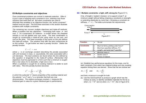
in which the subscript “o” means properties of the existing material and<br />
the asterisk * on Z* and α* is a reminder that both are now<br />
dimensionless. The relative exchange constant α * measures the<br />
fractional gain in value for a given fractional gain in performance.<br />
<strong>CES</strong> <strong>EduPack</strong> <strong>–</strong> <strong>Exercises</strong> <strong>with</strong> <strong>Worked</strong> <strong>Solutions</strong><br />
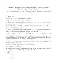
E8.1 Multiple constraints: a light, stiff, strong tie (Figure E11).<br />
A tie, of length L loaded in tension, is to support a load F, at<br />
minimum weight <strong>with</strong>out failing (implying a constraint on strength)<br />
or extending elastically by more than δ (implying a constraint on<br />
stiffness, F / δ ). The table summarises the requirements.<br />
Function • Tie rod<br />
Figure E11<br />
Constraints • Must not fail by yielding under force F<br />
• Must have specified stiffness, F/δ<br />
• Length L and axial load F specified<br />
Objective • Minimize mass m<br />
Free variables • Section area A<br />
• Choice of material<br />
(a) Establish two performance equations for the mass, one for<br />
each constraint, from which two material indices and one coupling<br />
equation linking them are derived. Show that the two indices are<br />
ρ<br />
M 1 = and<br />
E<br />
M.F. Ashby 2010 34 www.grantadesign.com/education/resources<br />
M 2<br />
ρ<br />
=<br />
σ y<br />
and that a minimum is sought for both.<br />
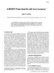
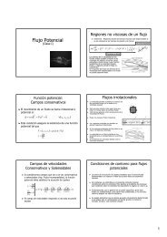
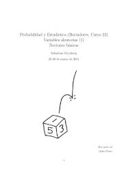
(b) Use the <strong>CES</strong> <strong>EduPack</strong> to produce a graph which has the<br />
indices as axes, to identify candidate materials for the tie (i)<br />
when δ /L = 10 -3 and (ii) when δ /L = 10 -2 , like in Figure E12.
Figure E12<br />
Answer. The derivation of performance equations and the indices they contain is laid out here:<br />
Objective Constraints Performance equation Index<br />
m = A L ρ<br />
Substitute for A<br />
Stiffness constraint<br />
Substitute for A<br />
F =<br />
δ<br />
Strength constraint F = σ y A<br />
E<br />
L<br />
A<br />
<strong>CES</strong> <strong>EduPack</strong> <strong>–</strong> <strong>Exercises</strong> <strong>with</strong> <strong>Worked</strong> <strong>Solutions</strong><br />
2 F ⎛ ρ ⎞<br />
m1<br />
= L ⎜ ⎟<br />
δ ⎝ E ⎠<br />
m2<br />
=<br />
L F<br />
⎛ ⎞<br />
⎜ ρ ⎟<br />
⎜ ⎟<br />
⎝<br />
σ y ⎠<br />
ρ<br />
M 1 = (1)<br />
E<br />
ρ<br />
= (2)<br />
σ y<br />
M.F. Ashby 2010 35 www.grantadesign.com/education/resources<br />
M 2
(The symbols have their usual meanings: A = area, L= length,<br />
ρ = density, F/δ =stiffness, E = Young’s modulus, σ y = yield<br />
strength or elastic limit.)<br />
The coupling equation is found by equating m1 to m2, giving<br />
⎛ ⎞<br />
⎜ ρ ⎟ L ⎛ ρ ⎞<br />
= ⎜ ⎟<br />
⎜ ⎟<br />
⎝<br />
σ y ⎠<br />
δ ⎝ E ⎠<br />
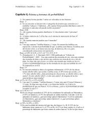
defining the coupling constant Cc = L/δ. The chart below shows<br />
the positions of the coupling line when L/δ = 100 and when L/δ =<br />
10 3 (corresponding to the required values of δ /L in the question)<br />
and the materials that are the best choice for each.<br />
δ -3<br />
= 10<br />
L<br />
δ -2<br />
= 10<br />
L<br />
Coupling<br />
lines<br />
<strong>CES</strong> <strong>EduPack</strong> <strong>–</strong> <strong>Exercises</strong> <strong>with</strong> <strong>Worked</strong> <strong>Solutions</strong><br />
Coupling<br />
condition<br />
Material choice Comment<br />
L/δ = 100 Ceramics: boron carbide,<br />
silicon carbide<br />
L/δ = 1000 Composites: CFRP; after<br />
that, Ti, Al and Mg alloys<br />
These materials are<br />
available as fibers as well<br />
as bulk.<br />
If ductility and toughness<br />
are also required, the<br />
metals are the best choice.<br />
The use of ceramics for a tie, which must carry tension, is<br />
normally ruled out by their low fracture toughness <strong>–</strong> even a small<br />
flaw can lead to brittle failure. But in the form of fibers both boron<br />
carbide and silicon carbide are used as reinforcement in<br />
composites, where they are loaded in tension, and their stiffness<br />
and strength at low weight are exploited.<br />
The <strong>CES</strong> <strong>EduPack</strong> software allows the construction of charts<br />
<strong>with</strong> axes that are combinations of properties, like those of ρ / E<br />
and ρ / σ y shown here, and the application of a selection box to<br />
identify the optimum choice of material.<br />
M.F. Ashby 2010 36 www.grantadesign.com/education/resources
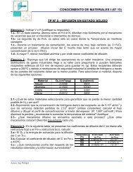
E8.2 Multiple constraints: a light, safe, pressure vessel (Figure<br />
E13) When a pressure vessel has to be mobile; its weight<br />
becomes important. Aircraft bodies, rocket casings and liquidnatural<br />
gas containers are examples; they must be light, and at the<br />
same time they must be safe, and that means that they must not<br />
fail by yielding or by fast fracture. What are the best materials for<br />
their construction? The table summarizes the requirements.<br />
Function • Pressure vessel<br />
Constraints • Must not fail by yielding<br />
• Must not fail by fast fracture.<br />
• Diameter 2R and pressure<br />
difference ∆ p specified<br />
Objective • Minimize mass m<br />
Free variables • Wall thickness, t<br />
• Choice of material<br />
(a) Write, first, a performance equation for the mass m of the<br />
pressure vessel. Assume, for simplicity, that it is spherical, of<br />
specified radius R, and that the wall thickness, t (the free variable)<br />
is small compared <strong>with</strong> R. Then the tensile stress in the wall is<br />
σ =<br />
∆p<br />
R<br />
2 t<br />
Figure E13<br />
<strong>CES</strong> <strong>EduPack</strong> <strong>–</strong> <strong>Exercises</strong> <strong>with</strong> <strong>Worked</strong> <strong>Solutions</strong><br />
where ∆ p , the pressure difference across this wall, is fixed by the<br />
design. The first constraint is that the vessel should not yield <strong>–</strong><br />
that is, that the tensile stress in the wall should not exceed σy. The<br />
second is that it should not fail by fast fracture; this requires that<br />
the wall-stress be less than K1c / π c , where K1c is the fracture<br />
toughness of the material of which the pressure vessel is made<br />
and c is the length of the longest crack that the wall might contain.<br />
Use each of these in turn to eliminate t in the equation for m; use<br />
the results to identify two material indices<br />
ρ<br />
= and<br />
σ y<br />
M.F. Ashby 2010 37 www.grantadesign.com/education/resources<br />
M 1<br />
ρ<br />
M 2 =<br />
K1c<br />
and a coupling relation between them. It contains the crack length,<br />
c.<br />
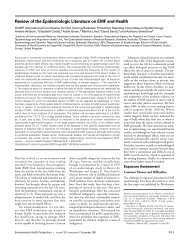
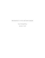
(b) Use the <strong>EduPack</strong> to produce a graph <strong>with</strong> the two material<br />
indices as axes, like in Figure E14. The coupling equation<br />
expresses the relationship between M1 and M2 and therefore Log<br />
M1 and Log M2 and can be plotted as a straight line on the Log<br />
M1<strong>–</strong>Log M2 chart. Determine the gradient and intercept of this line<br />
and plot it for first c= 5mm and then c= 5 µm. Identify the lightest<br />
candidate materials for the vessel for each case. M1 and M2 need<br />
to be minimised to find the lightest material.
Figure E14<br />
<strong>CES</strong> <strong>EduPack</strong> <strong>–</strong> <strong>Exercises</strong> <strong>with</strong> <strong>Worked</strong> <strong>Solutions</strong><br />
M.F. Ashby 2010 38 www.grantadesign.com/education/resources
Answer. The objective function is the mass of the pressure vessel:<br />
m = 4 π R<br />
2<br />
t ρ<br />
The tensile stress in the wall of a thin-walled pressure vessel (UASSP, 11) is<br />
∆p<br />
R<br />
σ =<br />
2 t<br />
<strong>CES</strong> <strong>EduPack</strong> <strong>–</strong> <strong>Exercises</strong> <strong>with</strong> <strong>Worked</strong> <strong>Solutions</strong><br />
Equating this first to the yield strength σ y , then to the fracture strength K1c / π c and substituting for t in<br />
the objective function leads to the performance equations and indices laid out below.<br />
Objective Constraints Performance equation Index<br />
∆pR<br />
Yield constraint σ ≤ σ y<br />
2 t<br />
Substitute for t<br />
m = 4 π R<br />
2<br />
t ρ<br />
Fracture constraint<br />
Substitute for t<br />
3 ⎡ ρ ⎤<br />
= m1<br />
= 2π<br />
∆p.R<br />
⋅ ⎢ ⎥<br />
⎣σy<br />
⎦<br />
∆pR<br />
K<br />
σ<br />
1c<br />
⎡ ⎤<br />
= ≤<br />
= ⋅<br />
3 ( ) 1/<br />
2 ρ<br />
m2 2π<br />
∆ p R πc<br />
⎢ ⎥<br />
2 t π c<br />
⎣ K1c<br />
⎦<br />
The coupling equation is found by equating m1 to m2, giving a relationship between M1 and M2:<br />
1/2<br />
M 1 = ( πc) M 2<br />
ρ<br />
= (1)<br />
σ y<br />
M.F. Ashby 2010 39 www.grantadesign.com/education/resources<br />
M 1<br />
ρ<br />
M 2 = (2)<br />
K1c<br />
On the (logarithmic) graph of the material indices, the coupling line therefore is log M1 = log (π c) 1/2 + log M2<br />
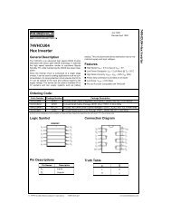
The position of the coupling line depends on the detection limit, c1 for cracks, through the term (π c) 1/2 .
The figure shows the appropriate chart <strong>with</strong> two coupling lines, one<br />
for c = 5 mm and the other for c = 5µm.<br />
The resulting selection is summarised in the table.<br />
Coupling condition Material choice<br />
from Figure E14<br />
Titanium alloys<br />
Crack length<br />
Aluminium alloys<br />
c ≤ 5 mm<br />
Steels<br />
( π c = 0.<br />
125 )<br />
Crack length<br />
c ≤ 5 µ m<br />
(<br />
π c = 3.<br />
96 x 10<br />
−3<br />
)<br />
CFRP<br />
Silicon carbide<br />
Silicon nitride<br />
Alumina<br />
Comment<br />
These are the standard<br />
materials for pressure<br />
vessels. Steels appear,<br />
despite their high density,<br />
because their toughness<br />
and strength are so high<br />
Ceramics, potentially, are<br />
attractive structural<br />
materials, but the difficulty<br />
of fabricating and<br />
maintaining them <strong>with</strong> no<br />
flaws greater than 5 µm is<br />
enormous<br />
Note: using the <strong>EduPack</strong> will reveal a wider range of candidate<br />
materials along the coupling lines.<br />
In large engineering structures it is difficult to ensure that there are<br />
no cracks of length greater than 1 mm; then the tough engineering<br />
alloys based on steel, aluminum and titanium are the safe choice. In<br />
the field of MEMS (micro electro-mechanical systems), in which films<br />
of micron-thickness are deposited on substrates, etched to shapes<br />
and then loaded in various ways, it is possible <strong>–</strong> even <strong>with</strong> brittle<br />
ceramics <strong>–</strong> to make components <strong>with</strong> no flaws greater than 1 µm in<br />
size. In this regime, the second selection given above has<br />
relevance.<br />
<strong>CES</strong> <strong>EduPack</strong> <strong>–</strong> <strong>Exercises</strong> <strong>with</strong> <strong>Worked</strong> <strong>Solutions</strong><br />
Coupling line,<br />
c = 5 microns<br />
Coupling line,<br />
c = 5 mm<br />
M.F. Ashby 2010 40 www.grantadesign.com/education/resources
E8.3 A cheap column that must not buckle<br />
or crush (Figure E15). The best choice of<br />
material for a light strong column depends<br />
on its aspect ratio: the ratio of its height H<br />
to its diameter D. This is because short, fat<br />
columns fail by crushing; tall slender<br />
columns buckle instead. Derive two<br />
performance equations for the material cost<br />
of a column of solid circular section and<br />
specified height H, designed to support a<br />
load F large compared to its self-load, one<br />
using the constraints that the column must<br />
not crush, the other that it must not buckle.<br />
The table summarizes the needs.<br />
Function • Column<br />
Constraints • Must not fail by compressive crushing<br />
• Must not buckle<br />
• Height H and compressive load F specified.<br />
Objective • Minimize material cost C<br />
Free variables • Diameter D<br />
• Choice of material<br />
(a) Proceed as follows<br />
Figure E15<br />
(1) Write down an expression for the material cost of the column <strong>–</strong> its<br />
mass times its cost per unit mass, Cm.<br />
(2) Express the two constraints as equations, and use them to<br />
substitute for the free variable, D, to find the cost of the column<br />
that will just support the load <strong>with</strong>out failing by either mechanism<br />
(3) Identify the material indices M1 and M2 that enter the two equations<br />
for the mass, showing that they are<br />
<strong>CES</strong> <strong>EduPack</strong> <strong>–</strong> <strong>Exercises</strong> <strong>with</strong> <strong>Worked</strong> <strong>Solutions</strong><br />
⎛ C ⎞<br />
= ⎜ m ρ ⎡C<br />
⎤<br />
M 1 ⎟<br />
⎜ ⎟<br />
and =<br />
m ρ<br />
M 2 ⎢ ⎥<br />
⎝ σ c<br />
1/2<br />
⎠<br />
⎣ E ⎦<br />
where C m is the material cost per kg, ρ the material density, σ c<br />
its crushing strength and E its modulus.<br />
(b) Data for six possible candidates for the column are listed in<br />
the Table. Use these to identify candidate materials when F = 10 5<br />
N and H = 3m. Ceramics are admissible here, because they have<br />
high strength in compression.<br />
Data for candidate materials for the column<br />
Material Density ρ<br />
(kg/m 3 )<br />
Wood (spruce)<br />
Brick<br />
Granite<br />
Poured concrete<br />
Cast iron<br />
Structural steel<br />
Al-alloy 6061<br />
Cost/kg<br />
Cm ($/kg)<br />
Modulus<br />
E (MPa)<br />
Compression<br />
strength<br />
σ c (MPa)<br />
M.F. Ashby 2010 41 www.grantadesign.com/education/resources<br />
700<br />
2100<br />
2600<br />
2300<br />
7150<br />
7850<br />
2700<br />
0.5<br />
0.35<br />
0.6<br />
0.08<br />
0.25<br />
0.4<br />
1.2<br />
10,000<br />
22,000<br />
20,000<br />
20,000<br />
130,000<br />
210,000<br />
69,000<br />
25<br />
95<br />
150<br />
13<br />
200<br />
300<br />
150<br />
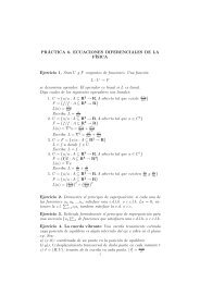
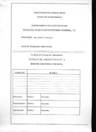
(c) Use the <strong>EduPack</strong> to produce a graph <strong>with</strong> the two indices as<br />
axes. Express M2 in terms of M1 and plot coupling lines for<br />
selecting materials for a column <strong>with</strong> F = 10 5 N and H = 3m (the<br />
same conditions as above), and for a second column <strong>with</strong> F = 10 3<br />
N and H = 20m.
Figure E16<br />
<strong>CES</strong> <strong>EduPack</strong> <strong>–</strong> <strong>Exercises</strong> <strong>with</strong> <strong>Worked</strong> <strong>Solutions</strong><br />
Answer. This, and exercises E 8.1 and E 8.2 illustrate the method of<br />
solving over-constrained problems. This one concerns materials for a<br />
light column <strong>with</strong> circular section which must neither buckle nor crush<br />
under a design load F.<br />
The cost, C, is to be minimised<br />
π<br />
C = D<br />
2<br />
H Cmρ<br />
4<br />
where D is the diameter (the free variable) and H the height of the<br />
column, Cm is the cost per kg of the material and ρ is its density. The<br />
column must not crush, requiring that<br />
4F<br />
≤ σ<br />
2<br />
c<br />
π D<br />
where σc is the compressive strength. Nor must it buckle:<br />
π<br />
2<br />
EI<br />
F ≤<br />
2<br />
H<br />
The right-hand side is the Euler buckling load in which E is Young’s<br />
modulus. The second moment of area for a circular column is<br />
π<br />
I = D<br />
4<br />
64<br />
The subsequent steps in the derivation of performance equations are<br />
laid out on the next page:<br />
M.F. Ashby 2010 42 www.grantadesign.com/education/resources
Objective Constraint Performance equation<br />
π<br />
C = D<br />
2<br />
H Cmρ<br />
4<br />
<strong>CES</strong> <strong>EduPack</strong> <strong>–</strong> <strong>Exercises</strong> <strong>with</strong> <strong>Worked</strong> <strong>Solutions</strong><br />
2<br />
π D<br />
⎡C<br />
⎤<br />
Crushing constraint F f ≤ σ c<br />
=<br />
m ρ<br />
C1<br />
F H ⎢ ⎥ (1)<br />
4<br />
⎣ σ c ⎦<br />
Buckling constraint<br />
2 3 4<br />
π EI π D E<br />
2 ⎡ ⎤<br />
F ≤ =<br />
=<br />
1/2 2 Cm<br />
ρ<br />
C<br />
H<br />
2<br />
64 H<br />
2<br />
2 F H<br />
1/2<br />
⎢<br />
1/2<br />
⎥ (2)<br />
π<br />
⎣ E ⎦<br />
⎡C<br />
⎤<br />
The first performance equation contains the index =<br />
m ρ<br />
M 1 ⎢ ⎥<br />
⎣ σ c ⎦<br />
, the second, the index<br />
⎡C<br />
⎤<br />
=<br />
m ρ<br />
M 2 ⎢<br />
1/2<br />
⎥ . This is a min-max problem: we seek the material <strong>with</strong> the lowest (min) cost C<br />
⎣ E ⎦<br />
~<br />
which itself is the larger (max) of C1 and C2. The two performance equations are evaluated in<br />
the Table, which also lists C max(<br />
C , C ).<br />
~<br />
= 1 2 for a column of height H = 3m, carrying a load F =<br />
10 5 N. The cheapest choice is concrete.<br />
Material Density ρ<br />
(kg/m 3 )<br />
Wood (spruce)<br />
Brick<br />
Granite<br />
Poured concrete<br />
Cast iron<br />
Structural steel<br />
Al-alloy 6061<br />
Substitute for D<br />
Substitute for D<br />
700<br />
2100<br />
2600<br />
2300<br />
7150<br />
7850<br />
2700<br />
Cost/kg<br />
Cm ($/kg)<br />
0.5<br />
0.35<br />
0.6<br />
0.08<br />
0.25<br />
0.4<br />
1.2<br />
Modulus<br />
E (MPa)<br />
10,000<br />
22,000<br />
20,000<br />
20,000<br />
130,000<br />
210,000<br />
69,000<br />
Compressio<br />
n<br />
strength<br />
σc (MPa)<br />
25<br />
95<br />
150<br />
13<br />
200<br />
300<br />
150<br />
M.F. Ashby 2010 43 www.grantadesign.com/education/resources<br />
C1<br />
$<br />
4.2<br />
2.3<br />
3.1<br />
4.3<br />
2.6<br />
3.0<br />
6.5<br />
C2<br />
$<br />
11.2<br />
16.1<br />
35.0<br />
4.7<br />
16.1<br />
21.8<br />
39.5<br />
C ~<br />
$<br />
11.2<br />
16.1<br />
35.0<br />
4.7<br />
16.1<br />
21.8<br />
39.5
The coupling equation is found by equating C1 to C2 giving<br />
1 / 2<br />
π<br />
1/2 ⎛ F ⎞<br />
M 2 = ⋅⎜<br />
⎟ ⋅ M<br />
2<br />
1<br />
2 ⎜ ⎟<br />
log M 2 = log M 1 + log<br />
⎝ H ⎠<br />
<strong>CES</strong> <strong>EduPack</strong> <strong>–</strong> <strong>Exercises</strong> <strong>with</strong> <strong>Worked</strong> <strong>Solutions</strong><br />
1/2<br />
π ⎛ ⎞<br />
⋅ ⎜ 2 ⎟<br />
2 ⎝ H ⎠<br />
F<br />
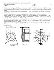
It contains the structural loading coefficient F/H 2 . Two positions for the coupling line are shown, one<br />
corresponding to a low value of F/H 2 = 0.011 MN/m 2 (F = 10 5 N, H = 3 m) and to a high one F/H 2 =<br />
2.5 MN/m 2 (F = 10 7 N, H = 2 m), <strong>with</strong> associated solutions. Remember that, since E and σ c are<br />
measured in MPa, the load F must be expressed in units of MN. The selection is listed in the table.<br />
Large F/H 2<br />
Small F/H 2<br />
Couplin<br />
g<br />
M.F. Ashby 2010 44 www.grantadesign.com/education/resources<br />
1/<br />
2
E8.4 An air cylinder for a truck (Figure E17). Trucks rely on<br />
compressed air for braking and other power-actuated systems. The air<br />
is stored in one or a cluster of cylindrical pressure tanks like that shown<br />
here (length L, diameter 2R, hemispherical ends). Most are made of<br />
low-carbon steel, and they are heavy. The task: to explore the<br />
potential of alternative materials for lighter air tanks, recognizing the<br />
there must be a trade-off between mass and cost <strong>–</strong> if it is too<br />
expensive, the truck owner will not want it even if it is lighter. The table<br />
summarizes the design requirements.<br />
Function • Air cylinder for truck<br />
Constraints • Must not fail by yielding<br />
• Diameter 2R and length L specified, so the<br />
ratio Q = 2R/L is fixed.<br />
Objectives • Minimize mass m<br />
• Minimize material cost C<br />
Free variables • Wall thickness, t<br />
• Choice of material<br />
(a) Show that the mass and material cost of the tank relative to one<br />
made of low-carbon steel are given by<br />
m<br />
mo<br />
⎛ ⎞⎛<br />
⎞<br />
⎜ ρ σ<br />
⎟⎜<br />
y,<br />
o<br />
=<br />
⎟<br />
⎜ ⎟⎜<br />
⎟<br />
⎝<br />
σ y ⎠⎝<br />
ρo<br />
⎠<br />
Figure E17<br />
and<br />
C<br />
Co<br />
⎛ ⎞⎛<br />
⎞<br />
⎜ Cm ρ σ<br />
⎟⎜<br />
y,<br />
o<br />
=<br />
⎟<br />
⎜ ⎟⎜<br />
⎟<br />
⎝<br />
σ y ⎠⎝<br />
Cm,<br />
o ρo<br />
⎠<br />
<strong>CES</strong> <strong>EduPack</strong> <strong>–</strong> <strong>Exercises</strong> <strong>with</strong> <strong>Worked</strong> <strong>Solutions</strong><br />
where ρ is the density, σy the yield strength and Cm the cost per kg<br />
of the material, and the subscript “o” indicates values for mild<br />
steel.<br />
(b) Explore the trade-off between relative cost and relative mass,<br />
considering the replacement of a mild steel tank <strong>with</strong> one made,<br />
first, of low alloy steel, and, second, one made of filament-wound<br />
CFRP, using the material properties in the table below. Define a<br />
relative penalty function<br />
* * m C<br />
Z = α +<br />
mo<br />
Co<br />
where α * is a relative exchange constant, and evaluate Z * for α * =<br />
1 and for α * = 100.<br />
Material Density ρ<br />
(kg/m 3 )<br />
Mild steel<br />
Low alloy steel<br />
CFRP<br />
Yield strength<br />
σc (MPa)<br />
314<br />
775<br />
760<br />
Price per /kg<br />
Cm ($/kg)<br />
0.66<br />
0.85<br />
42.1<br />
M.F. Ashby 2010 45 www.grantadesign.com/education/resources<br />
7850<br />
7850<br />
1550<br />
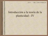
(c) Use the <strong>EduPack</strong> to produce a graph <strong>with</strong> axes of m/mo and C/Co,<br />
like the one in Figure E18 below. Mild steel (here labelled “Low<br />
carbon steel”) lies at the co-ordinates (1,1).<br />
Sketch a trade-off surface and plot contours of Z * that are<br />
approximately tangent to the trade-off surface for α * = 1 and for α *<br />
= 100. What selections do these suggest?
Answer. (a) The mass m of the tank is<br />
m<br />
= 2π<br />
R L t + 4π<br />
R<br />
2<br />
t = 2πR<br />
L t (<br />
1 +<br />
where Q, the aspect ratio 2R/L, is fixed by the design requirements. The<br />
stress in the wall of the tank caused by the pressure p must not exceed σ y ,<br />
is the yield strength of the material of the tank wall, meaning that<br />
p R<br />
σ = ≤ σ y<br />
t<br />
Figure E18<br />
Substituting for t, the free variable, gives<br />
Q )<br />
<strong>CES</strong> <strong>EduPack</strong> <strong>–</strong> <strong>Exercises</strong> <strong>with</strong> <strong>Worked</strong> <strong>Solutions</strong><br />
m<br />
=<br />
⎛ ⎞<br />
2<br />
⎜ ρ<br />
2π<br />
R L p ( 1 + Q ) ⎟<br />
⎜ ⎟<br />
⎝<br />
σ y ⎠<br />
The material cost C is simply the mass m times the cost per kg of the<br />
material, C m, giving<br />
C<br />
=<br />
Cm<br />
m<br />
M.F. Ashby 2010 46 www.grantadesign.com/education/resources<br />
=<br />
⎛ ⎞<br />
2<br />
⎜<br />
Cm<br />
ρ<br />
2π<br />
R L p ( 1 + Q ) ⎟<br />
⎜ ⎟<br />
⎝<br />
σ y ⎠<br />
from which the mass and cost relative to that of a low-carbon steel<br />
(subscript “o”) tank are<br />
m<br />
mo<br />
C<br />
Co<br />
⎛ ⎞⎛<br />
⎞<br />
⎜ ρ σ<br />
⎟⎜<br />
y,<br />
o<br />
=<br />
⎟<br />
⎜ ⎟⎜<br />
⎟<br />
⎝<br />
σ y ⎠⎝<br />
ρo<br />
⎠<br />
⎛ ⎞⎛<br />
⎞<br />
⎜ Cm ρ σ<br />
⎟⎜<br />
y,<br />
o<br />
=<br />
⎟<br />
⎜ ⎟⎜<br />
⎟<br />
⎝<br />
σ y ⎠⎝<br />
Cm,<br />
o ρo<br />
⎠<br />
and<br />
(b) To get further we need a penalty function:. The relative penalty<br />
function<br />
* * m C<br />
Z = α +<br />
mo<br />
Co<br />
This is evaluated for Low alloy steel and for CFRP in the table below, for<br />
α * = 1 (meaning that weight carries a low cost premium) <strong>–</strong> Low alloy<br />
steel has by far the lowest Z * . But when it is evaluated for α * = 100<br />
(meaning that weight carriers a large cost premium), CFRP has the<br />
lowest Z * .<br />
(c) The figure shows the trade-off surface. Materials on or near this<br />
surface have attractive combinations of mass and cost. Several are<br />
better low-carbon steel. Two contours of Z * that just touch the trade-off<br />
line are shown, one for α * = 1, the other for α * = 100 <strong>–</strong> they are curved<br />
because of the logarithmic axes.<br />
The first, for α * = 1 identifies higher strength steels as good choices.<br />
This is because their higher strength allows a thinner tank wall. The<br />
contour for α * = 100 touches near CFRP, aluminum and magnesium<br />
alloys <strong>–</strong> if weight saving is very highly valued, these become attractive<br />
solutions.
Material Density ρ<br />
(kg/m 3 )<br />
Mild steel<br />
Low alloy steel<br />
CFRP<br />
7850<br />
7850<br />
1550<br />
Yield strength<br />
σc (MPa)<br />
314<br />
775<br />
760<br />
Price per /kg<br />
Cm ($/kg)<br />
0.66<br />
0.85<br />
42.1<br />
Z* <strong>with</strong> α* = 1 Z* <strong>with</strong> α* = 100<br />
<strong>CES</strong> <strong>EduPack</strong> <strong>–</strong> <strong>Exercises</strong> <strong>with</strong> <strong>Worked</strong> <strong>Solutions</strong><br />
Z * ,<br />
α * = 1<br />
2<br />
1.03<br />
5.2<br />
Z * ,<br />
α * = 100<br />
101<br />
45.6<br />
13.4<br />
M.F. Ashby 2010 47 www.grantadesign.com/education/resources<br />
*