Tutorial for creating an Expert Choice model
Tutorial for creating an Expert Choice model
Tutorial for creating an Expert Choice model

Create successful ePaper yourself
Turn your PDF publications into a flip-book with our unique Google optimized e-Paper software.
TUTORIAL FOR ANALYTIC HIERARCHY PROCESS<br />
Structuring the decision <strong>model</strong><br />
The Analytic Hierarchy Process (AHP) is a general problem-solving<br />
method that is useful in making complex decisions (e.g., multi-criteria<br />
decisions) based on variables that do not have exact numerical consequences.<br />
We will explain the basics of <strong>creating</strong> <strong>an</strong>d using AHP <strong>model</strong>s.<br />
The software is supplied by <strong>Expert</strong> <strong>Choice</strong>, Inc., <strong>an</strong>d this tutorial is<br />
based on <strong>Expert</strong> <strong>Choice</strong>'s online tutorial. We encourage you to work<br />
through the online tutorial to get a fuller underst<strong>an</strong>ding of all the features<br />
of the AHP <strong>model</strong>.<br />
Decision <strong>model</strong>ing using <strong>Expert</strong> <strong>Choice</strong> (in the Evaluation <strong>an</strong>d<br />
<strong>Choice</strong> mode) typically consists of five steps: (1) Structuring the decision<br />
<strong>model</strong>, (2) Entering alternatives, (3) Establishing priorities among<br />
elements of the hierarchy, (4) Synthesizing, <strong>an</strong>d (5) Conducting sensitivity<br />
<strong>an</strong>alysis.<br />
You start by breaking down a complex decision problem into a<br />
hierarchical structure. You c<strong>an</strong> use the following elements: (1) Overall<br />
goal (subgoals) to be attained, (2) Criteria <strong>an</strong>d subcriteria, (3) Scenarios,<br />
<strong>an</strong>d (4) Alternatives.<br />
As <strong>an</strong> example, we will look at how a m<strong>an</strong>ager of <strong>an</strong> ice cream store<br />
chain decides where to open a new outlet. The goal is to select the better<br />
of two locations. The main criteria in this decision are (1) rental space<br />
cost, (2) traffic of potential customers, <strong>an</strong>d (3) the number of competitors.<br />
The store locations they are considering are a suburb<strong>an</strong> mall<br />
(moderate rent, high population of teenagers <strong>an</strong>d retirees who are known<br />
to be purchasers of ice cream) <strong>an</strong>d Main Street downtown (high rent,<br />
main traffic is office workers who are not around in the evenings <strong>an</strong>d on<br />
weekends).<br />
An <strong>Expert</strong> <strong>Choice</strong> <strong>model</strong> consists of a minimum of three levels: the<br />
overall goal of the decision at the top level, (sub)criteria at the second<br />
level, <strong>an</strong>d alternatives (the two locations <strong>for</strong> the store) at the third level.<br />
In <strong>model</strong>s with m<strong>an</strong>y levels, place the more general factors of the decision<br />
in the upper levels of the hierarchy <strong>an</strong>d the more specific criteria in<br />
the lower levels.
122<br />
Chapter 6 <strong>Tutorial</strong>s<br />
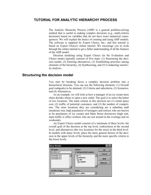
To start a new <strong>model</strong>, go to the <strong>Expert</strong> <strong>Choice</strong> File menu, <strong>an</strong>d<br />
choose New. Enter a name <strong>for</strong> the file in which to save the <strong>model</strong> you<br />
will build, e.g., location.ec1, <strong>an</strong>d click OK.<br />
To set up the <strong>model</strong> node by node, click Direct.<br />
Type in a description of the goal of the decision, e.g., “Select Site<br />
Location <strong>for</strong> new Ice Cream Outlet.”<br />
Click OK.<br />
For this example, the decision criteria are extent of competition<br />
(COMPET'N), customer fit (CUST FIT), <strong>an</strong>d cost (COST). To enter the<br />
criteria, go to the Edit menu <strong>an</strong>d choose Insert. This adds a level to the<br />
hierarchy directly below the active GOAL node. When you enter each<br />
criterion, e.g., COMPET'N, the program also allows you to give a description<br />
of the criterion, e.g., the number of competitors in the area.<br />
When you have entered in<strong>for</strong>mation about all the nodes at this level of<br />
the hierarchy, press .
Entering alternatives<br />
Analytic Hierarchy Process<br />
123<br />
To enter the alternatives, first select the COMPET'N node. Next, on the<br />
Edit menu, choose Insert. Type <strong>an</strong> abbreviation (eight characters or<br />
less) <strong>for</strong> the first alternative, e.g., Mall. You c<strong>an</strong> again enter a more detailed<br />
description <strong>for</strong> the alternative, e.g., “Suburb<strong>an</strong> mall location.”<br />
Click OK to enter the next alternative. When you have entered all alternatives,<br />
press .<br />
Activate the (sub)criterion node under which you entered the<br />
alternatives, go to the Edit menu <strong>an</strong>d choose Replicate children of<br />
current node.<br />
Click To Peers or To All Leaves to replicate the alternatives to all<br />
of the other nodes at the bottom of the <strong>model</strong>. Once the alternatives have
124<br />
Chapter 6 <strong>Tutorial</strong>s<br />
been associated with all subnodes, the alternatives will be displayed at<br />
the bottom of the screen.<br />
To save a <strong>model</strong>, go to the File menu <strong>an</strong>d choose Save.<br />
Establishing priorities among elements of the hierarchy<br />
Once you specified the decision <strong>model</strong> fully, you c<strong>an</strong> evaluate the<br />
alternatives <strong>an</strong>d criteria at each level to derive “local” priorities<br />
(weights) by making pairwise comparisons among elements at the same<br />
level in the hierarchy. First select the node <strong>for</strong> which you w<strong>an</strong>t to<br />
establish priorities. Go to the Assessment menu <strong>an</strong>d choose the<br />
assessment method, <strong>for</strong> example, Pairwise or Data.<br />
Entering import<strong>an</strong>ce weights (Assessment, Data:<br />
You c<strong>an</strong> enter absolute values <strong>for</strong> the weights of the nodes (instead of<br />
relative values such as those derived in the pairwise comparison mode),<br />
by clicking Assessment <strong>an</strong>d then Data. For example, you c<strong>an</strong> assign import<strong>an</strong>ce<br />
weights <strong>for</strong> the criteria competition, customer fit, <strong>an</strong>d cost, as<br />
shown below.
Analytic Hierarchy Process<br />
125<br />
After you enter the import<strong>an</strong>ce weights, click Calculate. The new<br />
values will be reflected in the decision <strong>model</strong>. (If the decision <strong>model</strong><br />
does not show the weights, click the P/F icon at the top of the screen.)<br />
Entering pairwise comparisons (Assessment, Pairwise)<br />
You c<strong>an</strong> make simple pairwise comparison judgments on each pair of<br />
items in the comparison set. To begin the pairwise assessment process,<br />
move to the first criterion by double-clicking on its node (e.g.,<br />
COMPT'N). Select Assessment <strong>an</strong>d then Pairwise (this is only available<br />
if there are nine alternatives or less) to compare the alternative sites on<br />
this criterion.<br />
Choose the type of comparison (Import<strong>an</strong>ce, Preference, Likelihood)<br />
<strong>an</strong>d the mode of comparison (Verbal, Graphical, Numerical).<br />
Choose a type <strong>an</strong>d mode that you feel com<strong>for</strong>table with. The type you<br />
select will not affect <strong>an</strong>y calculations per<strong>for</strong>med by Evaluation <strong>an</strong>d
126<br />
Chapter 6 <strong>Tutorial</strong>s<br />
<strong>Choice</strong> (the selected type will appear in the comparison statement). Generally,<br />
Import<strong>an</strong>ce is appropriate when comparing criteria, Preference<br />
is appropriate when comparing alternatives, <strong>an</strong>d Likelihood is appropriate<br />
when comparing uncertain events.<br />
Click OK. When only two nodes are to be compared, the Graphical<br />
comparison mode is the default.<br />
To indicate your preference in the graphical mode, click <strong>an</strong>d drag the<br />
upper or lower horizontal, judgment bars. Alternatively, you c<strong>an</strong> enter<br />
your assessment in the Verbal <strong>an</strong>d Numerical mode, in the Matrix<br />
mode, or Questionnaire mode. Choose the appropriate tab.<br />
When you have completed all of the comparisons, the program<br />
automatically calculates <strong>an</strong>d graphs the priorities <strong>an</strong>d gives you a measure<br />
of the inconsistency of your judgments (Inconsistency Ratio). (In our
Analytic Hierarchy Process<br />
127<br />
example, there is only one pairwise comparison, <strong>an</strong>d there<strong>for</strong>e no redund<strong>an</strong>t<br />
in<strong>for</strong>mation: the inconsistency measure is me<strong>an</strong>ingless.)<br />
Click Record to return to the main screen.<br />
Treat the other criteria in a similar fashion (e.g., double-click on the<br />
COST node) to continue the assessment process.<br />
After you finish making the pairwise comparisons <strong>an</strong>d evaluating the<br />
alternatives (at the lowest level of the hierarchy), compare the criteria<br />
pairwise with respect to the goal. The program uses this in<strong>for</strong>mation to<br />
derive the relative import<strong>an</strong>ce of the criteria (cost, customer fit, extent of<br />
competition).<br />
To make pairwise comparisons between criteria (instead of directly<br />
assigning import<strong>an</strong>ce weights earlier in “Entering Import<strong>an</strong>ce Weights”),<br />
double-click the GOAL node. Select Assessment <strong>an</strong>d then Pairwise to<br />
compare the criteria. Select Import<strong>an</strong>ce <strong>for</strong> the Type <strong>an</strong>d Verbal <strong>for</strong><br />
the comparison mode. Clicking Skip Preliminary Questions will bring<br />
you to the following screen:
128<br />
Synthesizing<br />
Chapter 6 <strong>Tutorial</strong>s<br />
Judge the relative import<strong>an</strong>ce of the two criteria <strong>an</strong>d click Enter to<br />
move to the next comparison. Click Calculate to get the measure of the<br />
inconsistency of your judgments.<br />
The Inconsistency Ratio is purely in<strong>for</strong>mational. The program does<br />
not en<strong>for</strong>ce consistency. It is unlikely that you will be perfectly consistent<br />
in making comparative judgments, particularly when dealing with<br />
int<strong>an</strong>gibles. As a rule of thumb, make the inconsistency ratio 0.10 or<br />
less. If you wish to improve the inconsistency ratio, go to the Assessment<br />
menu <strong>an</strong>d choose the Matrix mode. Pull down the Inconsistency<br />
menu <strong>an</strong>d select 1 most to see which is the most inconsistent judgment<br />
(highlighted cell). You c<strong>an</strong> enter a new judgment value – perhaps after<br />
looking at the “Best Fit” value that the system computes <strong>for</strong> reference<br />
purposes. You c<strong>an</strong> see this value by clicking the words Best Fit in the<br />
upper left of the matrix or going to the Inconsistency menu <strong>an</strong>d selecting<br />
Best Fit.<br />
When you have finished entering your judgments, click Record to<br />
save the values <strong>an</strong>d to return to the main screen.<br />
After you record your preferences, the program synthesizes the priorities<br />
across the hierarchy to calculate the final priorities of the alternatives.
Analytic Hierarchy Process<br />
129<br />
You c<strong>an</strong> choose between two numerical methods of synthesizing the<br />
data: the Distributive <strong>an</strong>d Ideal (default) Synthesis Modes.<br />
To synthesize, go to the Synthesis menu <strong>an</strong>d select From Goal.<br />
To see the list of the global priorities <strong>for</strong> all the hierarchy's nodes,<br />
click the Details button.<br />
You c<strong>an</strong> select the Distributive synthesis button, the Ideal synthesis<br />
button, or the Set button, which will lead you through a series of questions<br />
to determine the proper mode. The choice of the appropriate<br />
synthesis mode <strong>for</strong> <strong>an</strong> application depends on whether you view the decision<br />
situation as prioritizing among all the alternatives based on their<br />
relative worth (Distributive) or picking a single best alternative (Ideal).<br />
The ideal mode preserves the original r<strong>an</strong>ks as alternatives are added.<br />
The distributive mode allows r<strong>an</strong>ks to ch<strong>an</strong>ge. Allowing ch<strong>an</strong>ges in r<strong>an</strong>kings<br />
could me<strong>an</strong>, <strong>for</strong> example, that alternative A is preferred to<br />
alternative B be<strong>for</strong>e alternative C is introduced into the mix of alternatives<br />
being evaluated, but with the introduction of C, B becomes<br />
preferred to A. In the distributive mode, criteria weights depend on the<br />
degree to which each criterion differentiates between the alternatives being<br />
evaluated. This favors (i.e., assigns higher weights) to alternatives<br />
that are both better th<strong>an</strong> other alternatives on import<strong>an</strong>t criteria <strong>an</strong>d are<br />
unusual among the alternatives.<br />
We describe these two modes <strong>for</strong> synthesizing priorities below. For<br />
further in<strong>for</strong>mation <strong>an</strong>d examples, refer to the <strong>Expert</strong> <strong>Choice</strong> online help<br />
or tutorial.<br />
Distributive synthesis mode<br />
In the distributive synthesis mode, the program normalizes the weights<br />
of the alternatives under each criterion, i.e., it distributes the global<br />
weight of a criterion among the alternatives thereby dividing up the full<br />
criteria weight into proportions that correspond to the relative priorities<br />
of the alternatives. (The normalization is applied at all levels of the hierarchy<br />
up to the goal node.)
130<br />
Sensitivity <strong>an</strong>alysis<br />
Chapter 6 <strong>Tutorial</strong>s<br />
You should choose the distributive mode if you w<strong>an</strong>t your preferences<br />
<strong>for</strong> alternatives to depend on the number <strong>an</strong>d type of other<br />
alternatives being evaluated. Use the distributive mode when all the alternatives<br />
are relev<strong>an</strong>t, e.g., when the decision task calls <strong>for</strong> prioritizing<br />
alternatives, allocating resources, <strong>an</strong>d pl<strong>an</strong>ning when the r<strong>an</strong>king of the<br />
alternatives is affected by the other alternatives. In general, if the alternatives<br />
are distinct (i.e., not duplicates of each other) <strong>an</strong>d are well<br />
separated in their characteristics, you should use the distributive mode.<br />
Ideal synthesis mode<br />
In the ideal synthesis mode, the priorities of the alternatives are divided<br />
by the largest value among them <strong>an</strong>d then multiplied by the global<br />
weight of the given parent node. Consequently, the most preferred alternative<br />
in a group receives the entire group priority of the criterion<br />
immediately above it. The other alternatives receive a proportion of the<br />
global weight. (Note that if the same alternative is best <strong>for</strong> all the criteria,<br />
that alternative obtains <strong>an</strong> overall value of one, while the other<br />
alternatives obtain proportionately less. The sum <strong>for</strong> all the alternatives<br />
will be more th<strong>an</strong> one.) Unlike the distributive mode, the ideal mode<br />
maintains the r<strong>an</strong>k of the best alternative.<br />
The ideal mode is useful when the alternatives are not distinct <strong>an</strong>d<br />
you do not w<strong>an</strong>t the mere presence of copies or near-copies of alternatives<br />
to affect the decision outcome. For example, when comparing three<br />
computers, two low-priced computers are very similar to one <strong>an</strong>other<br />
<strong>an</strong>d the high-priced computer is better under most other criteria. The two<br />
low priced computers are both better alternatives with respect to cost,<br />
but they would cut into each others weight if the weight of cost is distributed<br />
among the alternatives (as is done in the distributive mode). The<br />
ideal mode would give the entire weight <strong>for</strong> cost to the cheapest computer,<br />
thereby making it a stronger competitor to the high-priced<br />
computer. The ideal mode divides the numerical r<strong>an</strong>ks of the alternatives<br />
<strong>for</strong> each criterion by the largest value among them, instead of normalizing<br />
the entire set. The most-preferred alternative receives the value of<br />
one. In this case, the r<strong>an</strong>ks of the alternatives do not depend on each<br />
other. Each new alternative added is compared only with the highest<br />
r<strong>an</strong>ked alternative <strong>for</strong> that criterion.<br />
In general, use the ideal mode when your sole concern is <strong>for</strong> the<br />
highest r<strong>an</strong>ked alternative <strong>an</strong>d the others do not matter, or when several<br />
alternatives have equal or very similar values along most criteria.<br />
To see distributive or ideal summary weights <strong>for</strong> alternatives, Click<br />
the Distributive or the Ideal button <strong>an</strong>d then click the Summary button.<br />
To see distributive or ideal weights <strong>for</strong> alternatives <strong>an</strong>d details, click<br />
the Distributive or the Ideal button <strong>an</strong>d then click the Details button.<br />
Use sensitivity <strong>an</strong>alysis to investigate how sensitive the r<strong>an</strong>kings of the<br />
alternatives are to ch<strong>an</strong>ges in the import<strong>an</strong>ce of the criteria. <strong>Expert</strong><br />
<strong>Choice</strong> offers five modes <strong>for</strong> graphical sensitivity <strong>an</strong>alysis:
� Per<strong>for</strong>m<strong>an</strong>ce<br />
� Dynamic<br />
� Gradient<br />
� Two-dimensional<br />
� Difference<br />
Analytic Hierarchy Process<br />
131<br />
Sensitivity <strong>an</strong>alysis from the Goal node will show the sensitivity of<br />
the alternatives with respect to the criteria below the goal. You c<strong>an</strong> also<br />
per<strong>for</strong>m sensitivity <strong>an</strong>alysis from nodes under the goal—provided the<br />
<strong>model</strong> has more th<strong>an</strong> three levels—to show the sensitivity of the alternatives<br />
with respect to lower-level criteria.<br />
To initiate the per<strong>for</strong>m<strong>an</strong>ce sensitivity <strong>an</strong>alysis, go to the sensitivitygraphs<br />
menu <strong>an</strong>d choose Per<strong>for</strong>m<strong>an</strong>ce.<br />
The criteria are represented by vertical bars, <strong>an</strong>d the alternatives are<br />
displayed as horizontal line graphs. The intersection of the alternative<br />
line graphs with the vertical criterion lines shows the priority of the alternative<br />
<strong>for</strong> the given criterion, as read from the right axis labeled Alt%.<br />
The criterion's priority is represented by the height of its bar as read<br />
from the left axis labeled Crit%. The overall priority of each alternative<br />
is represented on the OVERALL line, as read from the right axis.<br />
To per<strong>for</strong>m what-if <strong>an</strong>alysis, click a rect<strong>an</strong>gular criterion box <strong>an</strong>d<br />
drag it up or down to ch<strong>an</strong>ge the priority of that criterion. You c<strong>an</strong> observe<br />
the ch<strong>an</strong>ges this makes in the r<strong>an</strong>king of the alternatives on the<br />
right. In the above example, The Mall has higher overall priority (61 percent)<br />
even though it per<strong>for</strong>ms poorly on the Cost criterion.<br />
To restore the original priorities, press the key. Returning<br />
to the main menu also erases what-if ch<strong>an</strong>ges <strong>an</strong>d restores the priorities<br />
as originally calculated. You c<strong>an</strong> use the Window menu comm<strong>an</strong>d to
132<br />
Chapter 6 <strong>Tutorial</strong>s<br />
ch<strong>an</strong>ge to other sensitivity graphs. (What-if ch<strong>an</strong>ges will be reflected in<br />
the open windows only if you have not pressed the key.)<br />
There are other methods of investigating sensitivity using <strong>Expert</strong><br />
<strong>Choice</strong>:<br />
Dynamic sensitivity: The dynamic sensitivity <strong>an</strong>alysis is a horizontal<br />
bar graph that you c<strong>an</strong> use to increase or decrease the priority of <strong>an</strong>y criterion<br />
<strong>an</strong>d see the ch<strong>an</strong>ge in the priorities of the alternatives. For<br />
inst<strong>an</strong>ce, as you increase the CUST FIT criterion by dragging that bar to<br />
the right, the priorities of the remaining criteria decrease in proportion to<br />
their original priorities. The program recalculates the priorities of the alternatives<br />
based on their new relationship.<br />
Gradient sensitivity: The gradient sensitivity <strong>an</strong>alysis assigns each criterion<br />
a separate gradient graph. The vertical line represents the current<br />
priority of the selected criterion. The sl<strong>an</strong>ted lines represent the alternatives.<br />
The current priority of <strong>an</strong> alternative is where the alternative line<br />
intersects the vertical criterion line.<br />
2D Plot sensitivity: The two-dimensional plot sensitivity shows how<br />
well the alternatives per<strong>for</strong>m with respect to <strong>an</strong>y two criteria.<br />
Differences graph: The differences graph shows the differences between<br />
the priorities of the alternatives taken two at a time <strong>for</strong> all of the<br />
criteria. You c<strong>an</strong> go to the Options menu <strong>an</strong>d choose Weighted or Unweighted<br />
to show the differences in either m<strong>an</strong>ner. When unweighted,<br />
the criteria are treated as though they have equal priorities. When<br />
weighted, the criteria show both priorities <strong>an</strong>d differences.
Analytic Hierarchy Process<br />
JENNY’S GELATO CASE<br />
133<br />
Jennifer Edson was putting the finishing touches on the business pl<strong>an</strong> <strong>for</strong><br />
a new enterprise. Jenny’s Gelato, a retail establishment that will serve<br />
authentic Itali<strong>an</strong> gelato by the scoop or dish or <strong>for</strong> carryout. (Gelato is a<br />
rich, tasty ice cream sold in Italy.) Wholesale sales to restaur<strong>an</strong>ts in the<br />
Washington, D.C., Metro area were also included in the pl<strong>an</strong>. The business<br />
concept had been in Jennifer’s mind since she spent a semester<br />
abroad in Florence, Italy, during her undergraduate studies <strong>an</strong>d got<br />
“hooked” on gelato.<br />
Jennifer looked over the report <strong>an</strong>d everything seemed in order—it<br />
included everything from pro<strong>for</strong>ma fin<strong>an</strong>cial statements to taste test<br />
studies that she had conducted. A venture capitalist, in fact, thought the<br />
pl<strong>an</strong> was so good that she had obtained a verbal commitment <strong>for</strong> $50,000<br />
in start-up capital. Restaur<strong>an</strong>t equipment, store fixtures, <strong>an</strong>d gelatomaking<br />
machines had been comparison priced, <strong>an</strong>d she knew that these<br />
fixed costs would eat up the entire $5OK. Everything was “all systems<br />
go” <strong>for</strong> a summer opening save <strong>for</strong> the selection of a specific retail site.<br />
She felt that a downtown location was best because of the preponder<strong>an</strong>ce<br />
of Yuppies in the area. Negotiations <strong>for</strong> a specific site had come down to<br />
two alternatives, both of which involved leasing space.<br />
She had <strong>an</strong> option on <strong>an</strong> off-street site in the fashionable area of<br />
Georgetown in Washington, D.C. Twelve-hundred square feet of retailing<br />
space was available in a vac<strong>an</strong>t store whose only entr<strong>an</strong>ce was via <strong>an</strong><br />
alley off M Street (a street that was const<strong>an</strong>tly congested with pedestri<strong>an</strong><br />
<strong>an</strong>d auto traffic). The attractiveness of the Georgetown location was due<br />
principally to the heavy entertainment spot <strong>an</strong>d retail shopping traffic.<br />
Lots of weekday <strong>an</strong>d evening trade was available, as Georgetown was a<br />
haven <strong>for</strong> tourists arid college <strong>an</strong>d high school students. A long-term<br />
lease could be secured <strong>for</strong> $2500 a month but Jennifer would absorb<br />
nearly all the costs of converting the site to a twenty- to twenty-five seat<br />
gelateria. The option on the lease had to be exercised in two weeks.<br />
The alternative site was in <strong>an</strong> attractive, enclosed retailing <strong>an</strong>d office<br />
complex on Pennsylv<strong>an</strong>ia Avenue only five blocks from the White<br />
House. Shops in the minimall included restaur<strong>an</strong>ts, men’s <strong>an</strong>d women’s<br />
clothing stores, a jewelry store, a large record <strong>an</strong>d tape store, <strong>an</strong>d a series<br />
of international fast-food boutiques. The base <strong>for</strong> traffic was office<br />
workers within a three-block radius, <strong>an</strong>d faculty, staff <strong>an</strong>d students of a<br />
large urb<strong>an</strong> university whose buildings were all within three to four<br />
blocks of the complex. One thous<strong>an</strong>d square feet was available <strong>for</strong><br />
$2000 per month on a one-year lease, which would be renegotiated by<br />
the developer each year. The developer would also receive 2 percent of<br />
the businesses’ gross revenues. Since the location was new, the developer<br />
would custom build wall partitions <strong>an</strong>d arr<strong>an</strong>ge other space<br />
configurations to suit the ten<strong>an</strong>t.<br />
Jennifer developed a spreadsheet to summarize market research she<br />
had conducted on the two alternative sites (see Exhibit 1). She also pre-
134<br />
Chapter 6 <strong>Tutorial</strong>s<br />
pared a spreadsheet <strong>for</strong> the pro<strong>for</strong>ma income statement <strong>for</strong> the business<br />
(see Exhibit 2). Two of the assumptions underlying this latter spreadsheet<br />
were these:<br />
� The price per serving of gelato was $2.00<br />
� The cost of goods sold would be approximately 40 percent of the<br />
retail price<br />
Exhibit 2 also shows the results of a comparative breakeven <strong>an</strong>alysis<br />
on the two alternate sites. As expected, the higher fixed costs associated<br />
with the Georgetown site resulted in a higher breakeven point. Jennifer<br />
was unsure as to how much import<strong>an</strong>ce to attach to this <strong>an</strong>alysis because<br />
she felt that breakeven examined only downside risks. The real number<br />
she was most unsure about was <strong>for</strong>ecasted sales revenues <strong>for</strong> the first<br />
year of operations.<br />
Based on her review of trade <strong>an</strong>d academic sources, Jennifer developed<br />
the following mental <strong>model</strong> of factors that would influence sales of<br />
gelato at a retail site:<br />
Pennsylv<strong>an</strong>ia Avenue ‘M’ Street<br />
Criterion (Foggy Bottom) (Georgetown)<br />
Traffic<br />
(hourly pedestri<strong>an</strong> afternoon evening afternoon evening<br />
count) (noon-5 pm) (5-11 pm) (noon-5 pm) (5-11 pm)<br />
Monday 302 142 156 524<br />
Tuesday 286 202 215 426<br />
Wednesday 194 114 187 394<br />
Thursday 371 176 272 404<br />
Friday 226 224 413 735<br />
Saturday 75 110 521 816<br />
Sunday 62 90 795 692<br />
Total 1516 1058 2559 3991<br />
Average 216.6 151.1 365.6 570.1<br />
Average (afternoon &<br />
evening) 183.9 467.9<br />
EXHIBIT 1<br />
Pedestri<strong>an</strong> Traffic Count Study*<br />
*Each site storefront traffic counts taken during a single week in April. Traffic count is defined as pedestri<strong>an</strong>s passing<br />
by.
Analytic Hierarchy Process<br />
135<br />
Pennsylv<strong>an</strong>ia Avenue ‘M’ Street<br />
(Foggy Bottom) (Georgetown)<br />
Revenues $1,500,000 $1,500,000<br />
Cost of Goods Sold 600,000 600,000<br />
Gross Profit 900,000 900,000<br />
Rent 24,000 30,000<br />
L<strong>an</strong>dlord Percentage 30,000<br />
Depreciation 5,000 5,000<br />
Utilities 8,500 9,000<br />
General Overhead 50,000 50,000<br />
Advertising 100,000 100,000<br />
Site Preparation 0 20,000<br />
Licenses & Permits 1,500 1,500<br />
Total Operating Expenses $219,000 $229,000<br />
Net Profit<br />
Operating Profit $681,000 $671,000<br />
Interest Expense 9,000 9,000<br />
Taxable Profit 672,000 662,000<br />
Income Tax 248,640 244,940<br />
After Tax Profit $423,640 $417,060<br />
Breakeven Analysis<br />
Fixed Costs<br />
Rent $24,000 $30,000<br />
Depreciation 5,000 5,000<br />
Utilities 8,500 9,000<br />
General Overhead 50,000 50,000<br />
Interest 9,000 9,000<br />
Advertising 100,000 100,000<br />
Site Preparation Costs 0 20,000<br />
Total Fixed Costs $196,500 $223,000<br />
Variable Costs per Unit (scoop)<br />
Cost of Goods Sold $0.80 $0.80<br />
L<strong>an</strong>dlord Percentage 0.04 0.04<br />
Total Variable Costs $0.84 $0.80<br />
Contribution (per scoop) $1.16 $1.20<br />
Breakeven ($) $338,793 $371,667<br />
Breakeven (scoops) 169,397 185,833<br />
EXHIBIT 2<br />
Pro<strong>for</strong>ma Income Statement <strong>an</strong>d Breakeven Analysis<br />
� Sales of gelato would likely exhibit pronounced seasonal trends<br />
similar to those of regular ice cream, frozen yogurt, <strong>an</strong>d other frozen<br />
desserts.<br />
� Sales of gelato (like those of ice cream <strong>an</strong>d other frozen desserts)<br />
represent <strong>an</strong> unpl<strong>an</strong>ned, impulse type of buyer behavior.<br />
� Gelato <strong>an</strong>d other frozen desserts were often bought after consumers<br />
had participated in certain activities (after a movie, during a shopping<br />
trip, after participating in or watching a sporting event, after<br />
dinner at a restaur<strong>an</strong>t).
136<br />
Chapter 6 <strong>Tutorial</strong>s<br />
Criterion Pennsylv<strong>an</strong>ia Avenue (Foggy Bottom) ‘M’ Street (Georgetown).<br />
Building Br<strong>an</strong>d new office/retail Old row house converted to retail space complex<br />
Locale Enclosed minimall adjacent to PA Ave Freest<strong>an</strong>ding site in alleyway off M Street<br />
Ambi<strong>an</strong>ce Business offices, university Upscale shops, restaur<strong>an</strong>ts area<br />
Traffic Base State Dept., World B<strong>an</strong>k, government Tourists, college students, retail shoppers,<br />
employees, faculty, staff of university patrons of entertainment spots<br />
Avg. hourly<br />
traffic<br />
184 468<br />
Size 1000 sq. ft. 1200 sq. ft.<br />
Cost $2000 per month, developer takes 2 per- $2500 per month<br />
cent of <strong>an</strong>nual gross revenue<br />
Breakeven<br />
volume<br />
required<br />
Site develop- Subst<strong>an</strong>tial assist<strong>an</strong>ce from develmentoper/owner<br />
Competition Two ice-cream stores within a six-block<br />
radius of site<br />
EXHIBIT 3<br />
Comparison of Site Alternatives<br />
10 percent higher<br />
Lessee assumes all costs of improvement<br />
Five ice-cream stores within a six-block radius<br />
of site<br />
� Gelato dem<strong>an</strong>d would be higher among trendy, upscale yuppies<br />
who had cosmopolit<strong>an</strong> interests that often included experimenting<br />
with exotic, or so-called gourmet food.<br />
� Like m<strong>an</strong>y convenience retail concepts, sales <strong>for</strong> a gelateria<br />
would be heavily influenced by the volume of pedestri<strong>an</strong> traffic<br />
<strong>an</strong>d proximity to complementary retail businesses, restaur<strong>an</strong>ts,<br />
<strong>an</strong>d places of entertainment.<br />
� Competition from other ice-cream stores was <strong>an</strong> import<strong>an</strong>t factor—some<br />
malls, shopping areas <strong>an</strong>d other locations had reached<br />
the point of saturation or “overstoring.” The uniqueness of the<br />
gelato product, however, was expected to offset the heavy competition<br />
shown in traditional ice cream sales.<br />
These factors suggest that even though Jennifer Edson had done her<br />
homework with lots of conceptualization, fin<strong>an</strong>cial <strong>an</strong>alyses, <strong>an</strong>d<br />
observational studies she still had a complex problem on her h<strong>an</strong>ds in<br />
making the site-selection decision. Be<strong>for</strong>e she actually developed the<br />
<strong>Expert</strong> <strong>Choice</strong> <strong>model</strong> she decided to summarize the in<strong>for</strong>mation that she<br />
had collected about the characteristics of the two sites (see Exhibit 2).<br />
With this Jennifer Edson beg<strong>an</strong> the process of developing her <strong>Expert</strong><br />
<strong>Choice</strong> <strong>model</strong>.
EXERCISES<br />
Analytic Hierarchy Process<br />
137<br />
1. Construct <strong>an</strong> EC <strong>model</strong> similar to the one shown in Exhibit 4 to select<br />
the best retail site <strong>for</strong> the gelateria. (Make sure your criteria<br />
reflect both the qu<strong>an</strong>titative <strong>an</strong>d qualitative aspects of this problem.)<br />
2. Use EC’s sensitivity <strong>an</strong>alysis utility to per<strong>for</strong>m a what-if <strong>an</strong>alysis<br />
of the alternative. Document your assumptions.<br />
3. Provide a one-page report (excluding tables <strong>an</strong>d figures) summarizing<br />
your recommendations to Ms. Edson.<br />
Competition Competition at site.<br />
Condition Condition of Store<br />
Count Count of Traffic During Business Hours<br />
Drawing Power Drawing Power of Location <strong>for</strong> this Type of Retail Store<br />
Fin<strong>an</strong>cial Fin<strong>an</strong>cial Considerations<br />
Foggy Bottom Foggy Bottom Area of Washington, D.C.<br />
Georgetown Georgetown Area of Washington, D.C.<br />
L<strong>an</strong>dlord $ Percent of Sales Commission to l<strong>an</strong>dlord<br />
Lease $ Cost to lease<br />
Physical Physical Characteristics of Site<br />
Siteprep Outlay Required to Prepare Site<br />
Size Size of Store<br />
Traffic Traffic at Site<br />
Visible Visibility<br />
EXHIBIT 4<br />
EC Model <strong>for</strong> Retail-Site Selection: Select the Best Retail Site