University of California - Leif and Vera Svalgaard's

University of CaliforniaPeer ReviewedTitle:Effects of the Weak Polar Fields of Solar Cycle 23: Investigation Using OMNI for the STEREOMission PeriodAuthor:Lee, C. O.; Luhmann, J. G.; Zhao, X. P.; Liu, Y.; Riley, P.Arge, C. N. et al.Publication Date:04-09-2009Publication Info:Postprints, Multi-CampusPermalink:http://www.escholarship.org/uc/item/15v8k1wmCitation:Lee, C. O., Luhmann, J. G., Zhao, X. P., Liu, Y., Riley, P., Arge, C. N., et al.(2009). Effectsof the Weak Polar Fields of Solar Cycle 23: Investigation Using OMNI for the STEREO MissionPeriod. Solar Physics: A Journal for Solar and Solar-Stellar Research and the Study of SolarTerrestrial Physics, 256(1), pp 345-363. doi: 10.1007/s11207-009-9345-6. Retrieved from: http://www.escholarship.org/uc/item/15v8k1wmDOI:10.1007/s11207-009-9345-6Abstract:The current solar cycle minimum seems to have unusual properties that appear to be related toweak solar polar magnetic fields. We investigate signatures of this unusual polar field in the eclipticnear-Earth interplanetary magnetic field (IMF) for the STEREO period of observations. Using 1 AUOMNI data, we find that for the current solar cycle declining phase to minimum period the peak ofthe distribution for the values of the ecliptic IMF magnitude is lower compared to a similar phase ofthe previous solar cycle. We investigate the sources of these weak fields. Our results suggest thatthey are related to the solar wind stream structure, which is enhanced by the weak polar fields.The direct role of the solar field is therefore complicated by this effect, which redistributes the solarmagnetic flux at 1 AU nonuniformly at low to mid heliolatitudes.eScholarship provides open access, scholarly publishingservices to the University of California and delivers a dynamicresearch platform to scholars worldwide.

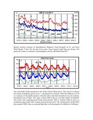
346 C.O. Lee et al.field in the ecliptic near-Earth interplanetary magnetic field (IMF) for the STEREO periodof observations. Using 1 AU OMNI data, we find that for the current solar cycle decliningphase to minimum period the peak of the distribution for the values of the ecliptic IMFmagnitude is lower compared to a similar phase of the previous solar cycle. We investigatethe sources of these weak fields. Our results suggest that they are related to the solar windstream structure, which is enhanced by the weak polar fields. The direct role of the solarfield is therefore complicated by this effect, which redistributes the solar magnetic flux at1 AU nonuniformly at low to mid heliolatitudes.Keywords STEREO mission · Solar wind · Solar cycle, models · Solar cycle,observations · Magnetic fields, observations · Magnetic fields, interplanetary1. IntroductionThe recent solar cycle 23 deep solar minimum period appears to be unlike previous onessince the dawn of the Space Age. The Sun, which has been spotless for over 200 daysin the year 2008, has weaker polar magnetic fields. The solar polar field values observedusing ground-based magnetographs are half their previous solar minimum values (see Figure1). This results in changes in the interplanetary medium. Measurements from the Ulyssesspacecraft (Balogh et al., 1992; Bameet al., 1992) fast-latitude scans reveal that the averageradial magnetic field values observed during the current minimum period are only abouttwo-thirds of their values measured during the previous minimum period (Smith and Balogh,2009). The related Ulysses plasma measurements reveal that the solar wind emanating fromthe large polar coronal holes is slightly slower, significantly less dense, and cooler, withless mass and momentum flux than previous solar minimum values (McComas et al., 2008;Issautier et al., 2008).In this study we examine the near-ecliptic solar wind and interplanetary magnetic field(IMF) at 1 AU for differences, if any, that exist as a direct result of the weaker solar polarfields of this cycle. We now know much more about the solar wind in terms of its differentFigure 1 Solar polar field strength versus time. The figure is adapted from the original on the StanfordWilcox Observatory Web site (http://wso.stanford.edu/gifs/Polar.gif). The blue (red) line represents the fieldstrength observed in the north (south); the thin (thick) black line represents the average (smoothed average).Note that the calibration of the y-axis is not very reliable since the measurements are obtained from the polewardbins of the magnetograph (see Svalgaard, Duvall, and Scherrer, 1978, for a discussion). Nevertheless,the overall trend is shown very well.

348 C.O. Lee et al.Figure 3 Histogram of occurrence at 1 AU for a solar minimum period spanning 10 CRs (see text forspecific CR ranges). The colors represent data from SC 23 (red) and SC 22 (black). Shown are histograms for(a) density, (b) velocity, and (c) momentum flux, N × V .Figure 4 (a) Histogram ofoccurrence for the magnetic fieldmagnitude observed over 10 CRsduring SC 22 (black) and 23(red). (b) Similar histogram forSTEREO-A (dark blue) andSTEREO-B (light blue)observations overplotted with SC23 (red).Figure 3(b) shows a similar histogram but for velocity. Both the SC 22 and 23 velocitydistributions have peak values occurring around 340 km s −1 . Notice that for SC 22 the percentoccurrence of this peak distribution is 40% greater than that for SC 23. For both periodsa high-speed tail distribution can be seen centered near 580 km s −1 , although the percent occurrenceis slightly larger for SC 23. Figure 3(c) shows the momentum flux (N × V )forthetwo solar cycle periods. For SC 23, the peak occurs around 1.25 cm −2 s −1 , which is about38% less than the peak value for the SC 22 period (2 cm −2 s −1 ). Note that the decrease inthe momentum flux during SC 23 is controlled by the density (see Figure 3(a)). This lowermomentum flux is consistent with recent findings by McComas et al. (2008) usingUlyssesdata from high heliolatitudes, although as will be discussed in the following, the source(s)differ.Figure 4(a) shows a histogram of the magnetic field magnitude. There is an overall shifttoward lower values in the distribution of the field magnitude during SC 23 in comparisonwith SC 22. The peak of the distribution for the SC 23 period is centered at 3.5 nT, which is30% less than 5 nT, the approximate central value for the peak of the SC 22 distribution.Figure 4(b) shows a comparison of the OMNI SC 23 observations with the 10-minuteresolutionSTEREO-A and STEREO-B magnetometer data (Acuña et al., 2008) obtainedfrom the STEREO in situ data Web site (http://www-ssc.igpp.ucla.edu/ssc/stereo/) hostedby the Institute of Geophysics and Planetary Physics at the University of California, LosAngeles (e.g., Luhmann et al., 2008). The STEREO observations exhibit the same lowerfield distribution as the OMNI data.To illustrate how the individual IMF components are contributing to the overall lowerfield magnitude during this current solar minimum period, we plot histograms of the standardRTN components. Figure 5(a) shows the histogram for the absolute values of the radialfield. The SC 23 distribution is shifted toward lower field values, with the peak occurrencecentered at 1.5 nT. The SC 22 distribution is slightly broader and has the peak occurrencecentered at 2.5 nT. For the SC 23 period, radial field values that are ≤3 nT occur more often,by ≈25%, than during the SC 22 period. Figure 5(b) shows a similar histogram, but for

Falls Creek Proposed Hydroelectric ProjectReconnaissance Reportstream gradient is 418 ftlmi and stream width averages 15 ft wide. The Falls Creek substrateincludes cobble, boulder deposits, few gravel bars and a thin layer of fine silt near the mouth; thelower one mile of stream has been extensively channelized and modified by placer mining (APA1984). Three to four acres adjacent to the active channel in the lower 0.5 miles are covered withtailings and 100 yards of the streambed in this area has been relocated (AEIDC 1982).The lower 2,300 ft of Falls Creek is classified as anadromous in the ADF&G AnadromousWaters Catalog (A WC). Anadromous fish species present in Falls Creek included juvenileChinook (Oncorhynchus tshawytscha) and juvenile Dolly Varden (Salve linus malma) (USFWS1961, Johnson and Daigneault 2008, AEIDC 1982).Previous StudiesThe hydroelectric potential at Grant Lake, approximately 1 mile north of Falls Creek, has beenevaluated several times as a potential power source for the SewardlKenai Peninsula area. In1954 R.W. Beck and Associates (cited in APA 1984) prepared a preliminary investigation andconcluded that a project was feasible. In 1980 CH2M Hill (cited in APA 1984) prepared a prefeasibilitystudy for a Grant Lake project and concluded that a project developed at the site wasfeasible.The most extensive study was performed by Ebasco Services, Inc. in 1984 for the Alaska PowerAuthority (APA 1984). Falls Creek (Figure 1) was investigated by Ebasco in 1984 for theAlaska Power Authority (now Alaska Energy Authority) as a possible source of additional flowsthat could be diverted to nearby Grant Lake in support of a hydroelectric project there (APA1984).Environmental ConsiderationsThe following presents a general overview of potential expected environmental considerationsfor a hydroelectric project at Falls Creek. This section describes fish resources, wetlands,hydrology and water quality, recreation, subsistence, and cultural resources of the project area.The area is managed using several specific management plans, including the Chugach NationalForest Plan (Meade 2006), Kenai River Comprehensive Management Plan (DNR 1998), andKenai Borough Coastal Management Plan (KPB 2008). Another search for all relevant landmanagement plans would be required as part of FERC licensing and by other required permittingprocesses.Ebasco (APA 1984) compiled a feasibility report on the Grant Lake hydroelectric project,including detailed environmental studies of water use and quality; aquatic, botanical and wildliferesources; historical and archaeological resources; socioeconomic impacts; geological and soilresources; recreational resources; aesthetic resources; and land use. The Arctic EnvironmentalData Center (AIEDC 1982 and 1983) and USFWS (1961) conducted environmental baselinestudies in the project area. For the purposes of this feasibility report, HDR Alaska did notconduct any environmental work beyond initial reconnaissance visits and instantaneous flowmeasurements (see Hydrology and Water Quality below) and this overview draws mainly onthese historical reports.2

350 C.O. Lee et al.Figure 7 (Top to bottom) Time series of the velocity, density, and field magnitude for the SC 23 time periodshown in Figures 3 and 4. The red values are data filtered for field magnitude values that are ≤4nT.related compression ridges. The association with the rise of the high-density ridges is alsovery pronounced.Figure 8 shows a similar set of time series for the SC 22 period. In comparison with theSC 23 period shown in Figure 7, the top panel of Figure 8 shows that there are generallyfewer high-speed streams during SC 22. As before, the red dots correspond to data thathave been filtered for field magnitudes ≤4 nT. The association of field magnitudes that are≤4 nT with the trailing part of the high-speed streams is not as clean when compared to thecurrent cycle (Figure 7, top panel). However, if we include data filtered for field magnitudesbetween 4 and 5 nT (shown in blue), the quality of the association is similar to what is shownfor SC 23.To examine in more detail the correlation between the velocity structures and the fieldmagnitudes observed at 1 AU over the SC 22 and 23 periods, we plot time series that areorganized by Carrington rotation and effectively stack them against each other to producecolor contour plots, as shown in Figures 9 and 10. Thex-axis displays the day of the CR(0 to 27), the y-axis displays the CR number (1893 – 1902 for SC 22 or 2053 – 2062 forSC 23), and the color represents the magnitude of the solar wind velocity (top panels) ortotal magnetic field (bottom panels). The black areas in the plots represent data gaps in theobservations.Figure 9 (top panel) shows the high-speed (red, orange) and low-speed (cyan, blue)stream structures, which were very prominent during the SC 23 period. For each Carringtonrotation, there were typically two high-speed and corresponding low-speed streams. Thebottom panel shows that the ridges of high magnetic field magnitudes (red) occur during therise of the high-speed streams (top panel, regions where the colors abruptly transition fromblue to red). In contrast, the ridges of low field magnitudes (blue) occur during the trailingpart of the high-speed streams (top panel, regions where the colors slowly transition fromyellow to green to blue).

Effects of the Weak Polar Fields of Solar Cycle 23 351Figure 8 (Top to bottom) Time series of the velocity, density, and field magnitude for the SC 22 time periodshowninFigures3 and 4. The blue (red) values are data filtered for field magnitude values that are between4and5nT(≤4nT).Figure 9 Color contour plot forthe SC 23 time period. Shown arecontours for (top panel) velocity(km s −1 ) and (bottom panel)magnetic field magnitude (nT).Figure 10 shows similar color contour plots, but for the SC 22 period. Although thereare high- and low-speed stream structures during this time period (see top panel), thehigh-speed streams are not as abundant and well organized as those observed during theSC 23 period. Also, the contrast between the high- and low-speed stream structures (redto blue) is not as great. For example, the high-speed structure observed during CR 1896on days 7 to 9 has a very gradual declining portion that lasts several days, where thespeeds decrease from ≈550 km s −1 (yellow – green) to ≈400 km s −1 (cyan) before the next

352 C.O. Lee et al.Figure 10 Color contour plotfor the SC 22 time period. Shownare contours for (top panel)velocity (km s −1 ) and (bottompanel) magnetic field magnitude(nT).high-speed stream structure commences on days 13 to 18. In contrast, the trailing part ofthe high-speed streams observed in the SC 23 period shows a more abrupt decline. Thespeeds go from ≈550 km s −1 (yellow – green) to ≈400 km s −1 in a day or so, followedby a sharp transition to speeds below 350 km s −1 (blue), which lasts for several days beforethe next high-speed stream onset. Figure 10 (bottom panel) shows the magnetic fieldmagnitude observed at this time. Notice that during SC 22 the field magnitudes have moremid-range (green to yellow) and high (red) field values and fewer low field values (blue)when compared to the current cycle. In addition, the ridges of high magnetic field magnitudes(red) do not necessarily occur during the onset of the high-speed streams, nordo the low field values always occur during the trailing part of the high-speed streams.We note that some solar transient events occurred during the time periods presented. Thenumber of interplanetary coronal mass ejections (ICMEs) observed during the SC 22 periodis eight compared to two during the SC 23 time period (see Jian et al., 2006, andhttp://www-ssc.igpp.ucla.edu/forms/stereo/stereo_level_3.html). This may in part explain theless organized nature of the SC 22 period.We also examine the correlation between the observed densities and field magnitudes.Figure 11 shows color contours of the statistics of the magnetic field magnitudes versusdensity. The maximum values in the distribution are shown in red. For the SC 22 distribution,Figure 11(a) shows that the maximum occurrence ranges between field magnitudesof around 4 – 6 nT and density values of around 2 – 6 cm −3 . For the SC 23 distribution(Figure 11(b)), the maximum occurrence distribution is shifted toward lower values in fieldmagnitude and broader in range, from approximately 2 to 5.5 nT. The density distribution isshifted toward lower values as well (about 1.5 – 6 cm −3 ). Overall, the recent SC 23 periodexhibits both lower field magnitudes and densities, consistent with the conclusions derivedfrom Figures 5 through 10.4. Origin of the Low IMFTo determine the nature of the differences in the present cycle interplanetary fields andtheir possible relationship to the weak solar polar fields mentioned in Section 1, itisnecessary to consider their origins. Although we do not show this, from the computed

Effects of the Weak Polar Fields of Solar Cycle 23 353Figure 11 Color contour plots of the magnetic field magnitude versus density for (a) SC 22 and (b) SC 23;(c) zoomed-in version of (a) and (d) zoomed-in version of (b).source surface coronal field maps available at the Wilcox Solar Observatory (WSO;http://wso.stanford.edu/synsourcel.html) the neutral line of the heliospheric current sheet(HCS) is seen to be more warped during CRs 2053 – 2062 in SC 23 in comparison withCRs 1893 – 1902 in SC 22. If the slow wind belt roughly follows the neutral line, the inferenceis that the stream structure should be more pronounced for the solar cycle minimum inSC 23, which we do observe, as shown in Figure 7 (top panel). The greater warping shouldmaximize the interaction between the high- and low-speed streams. In comparison, whenthe HCS is flat and near equatorial, as it is during the previous solar minimum, the streaminteractions are less well formed and the ecliptic intersection of them shows less contrast. Inparticular, the formation of rarefactions in the ecliptic is expected to be weaker, as suggestedby the results of Riley and Gosling (2007).The sources of the high-speed streams are also different for these two near-solar minimumperiods. Using the Wang – Sheeley – Arge (WSA) semiempirical solar wind model(Arge et al., 2004), we locate the sources of the high-speed streams observed at 1 AU.Standard plots used to map the solar wind sources with the WSA model are shown in Figures12 and 13 for several Carrington rotations from the periods under study. Here, thecolored regions are the predicted footpoints of the open field lines at the photosphere (i.e.,the coronal holes), where the colors indicate the solar wind speed at 21.5R ⊙ arising froma particular open field region, and the black lines indicate where the open regions are magneticallyconnected to the ecliptic plane. Figure 12 suggests that for the time period in SC22, the sources of the ecliptic solar wind streams are mostly polar coronal hole edges and

354 C.O. Lee et al.Figure 12 The derived coronal sources for CRs 1893 (top), 1895 (middle), and 1899 (bottom) using theWSA coronal model. The calculated footpoints (colored dots) of the open field lines at the photosphere areshown. The different colors indicate the solar wind speed (at 21R ⊙ ) associated with the flux tubes, whereasthe solid black lines connect the outer coronal boundary at 21.5R ⊙ and the source regions of the solar windat the photosphere. The + symbol indicates the daily position of the sub-Earth point on the Sun, which variesbetween ±7.25° in solar latitude owing to the inclination of solar rotation axis with respect to the eclipticplane. Note that the newest (oldest) data are located on the left side (right side).extensions. In contrast, Figure 13 shows that, for SC 23, most of the high-speed streamsoriginate from isolated open field sources located in the low- and mid-latitude regions. Itseems that there were very few comparable low- and mid-latitude holes supplying the highspeedwind during the SC 22 period. Extreme-ultraviolet (EUV) images from the Solarand Heliospheric Observatory (SOHO) Extreme ultraviolet Imaging Telescope (EIT) (Delaboudiniereet al., 1995) and STEREO Sun Earth Connection Coronal and HeliosphericInvestigation (SECCHI) Extreme UltraViolet Imager (EUVI) (Howard et al., 2002) confirmthis difference.To investigate the shapes and heliospheric extent of the high-speed stream sources, weconsider the global outward mapping of the various coronal holes that are supplying thesolar wind during the SC 22 and 23 periods. We use the potential field source surface (PFSS)approximation of the coronal field (cf. Schatten, Wilcox, and Ness, 1969) in the same manner

Effects of the Weak Polar Fields of Solar Cycle 23 355Figure 13 The derived coronal sources for CRs 2053 (top), 2058 (middle), and 2061 (bottom) using theWSA coronal model.as Zhao and Webb (2003) to map each derived open field region from the photosphere outto the source surface at 2.5R ⊙ (solar radii). Magnetograms from the WSO are used as inputto the PFSS model.Figure 14 (top panel) shows the open and closed field regions below 1.25R ⊙ for CR 1898during the SC 22 period. The solid black curve marks the magnetic neutral line, whereas thecolor dotted areas and the blue – red field lines indicate the open and closed field regions,respectively. Six regions of open field lines can be seen for CR 1898, as shown in differentcolors. Three regions are polar coronal hole (PCH) extensions, two are polar coronal holes,and one is an isolated low- to mid-latitude coronal hole. The second panel shows the variousphotospheric sources mapped to the source surface. Note that the colors correspond to thecolored regions shown in the top panel. The magnetic polarities of the open field regionsare indicated by the plus and minus symbols for open field pointing away from and towardthe Sun, respectively. For CR 1898, the four isolated and PCH extensions of open fieldregions map out to a moderate latitude range at the source surface. Dominating the sourcesurface map are open fields extending from within the PCH regions. The latitudinal extentof these open fields is wide, where some of the open fields map down to latitudes over

356 C.O. Lee et al.Figure 14 Global outward mapping of coronal holes supplying the solar wind for CR 1898 during theSC 22 period. (Top panel) Open (color dotted areas) and closed (areas with blue – red field lines) field regionsbelow 1.25R ⊙ . (Second panel) The photospheric sources mapped out to the source surface at 2.5R ⊙ .Thetwosolid gray bars mark the ecliptic plane location (between ±7.25° latitudes). The thick blue curve near the topof the panel marks the projected Ulysses trajectory. (Third panel) The WSA model predictions of the coronalhole areas and the solar wind speeds arising from them. (Bottom panel) The magnetic field magnitude at 1 AUmodeled by the coupled MAS/ENLIL solar wind model. The black curve seen throughout is the magneticneutral line.a broad longitude range within the ecliptic plane (between ±7.25° latitudes) as indicatedby the two solid gray bars. Other Carrington rotations from the SC 22 period of our studyalso show similar features, where the open fields from the PCHs have very wide latitudinalextents at the source surface and the isolated and PCH-extension regions of open fieldshave a moderate to narrow latitudinal range. This is consistent with the Ulysses results ofMcComas et al. (2008), who showed that the band of solar wind variability was narrowand confined to low latitudes during this period. The solid blue curve near the top of this

Effects of the Weak Polar Fields of Solar Cycle 23 357second panel marks the projected Ulysses trajectory for this Carrington rotation (data isfrom http://cohoweb.gsfc.nasa.gov/helios/heli.html).The third panel of Figure 14, similar to Figures 12 and 13, shows the WSA model predictionsof the coronal hole areas and the solar wind speeds arising from them. The crossesmark the daily position of the sub-Earth point on the Sun, providing information about wherethe solar wind observed at Earth is coming from on the Sun. For CR 1898, the majority ofthe medium- to high-speed winds in the ecliptic are coming from the PCH edges and extensions.Noteworthy are subtle differences between the top and third panels with regardto the open field areas, in terms of shapes, locations, etc. These differences arise becausethe PFSS model here uses magnetograms from WSO whereas the WSA model uses magnetogramsfrom the National Solar Observatory (NSO) (Henney, Keller, and Harvey, 2006)anda coupled coronal model consisting of the PFSS and Schatten current sheet model (Schatten,1971). However, these differences do not affect the basic information obtained from thesesource mappings.The bottom panel of Figure 14 shows the mapping of the magnetic field magnitudeat 1 AU based on the open field regions shown for CR 1898. The results are generatedby the coupled coronal MHD Around a Sphere (MAS) model (Riley, Linker,and Mikic, 2001), together with the ENLIL solar wind model (Odstrcil, 2003) (henceforthMAS/ENLIL). The coupled model uses NSO magnetograms and is publicly availablethrough the runs-on-request service at the Community Coordinated Modeling Center(CCMC) (http://ccmc.gsfc.nasa.gov). The colors shown are the field magnitude values in theunits of nanotesla, though it should be mentioned that the MAS/ENLIL solar wind modelvalues tend to be underestimated by a factor of ≈2 compared to observations (see Lee etal., 2009, for a discussion). The regions of low field magnitudes (patches of dark blue) areconfined to a narrow latitudinal range and usually coincide with the rarefaction regions inthe trailing parts of the high-speed streams (e.g., Figures 7 and 8), which in this case areconfined to fairly low latitudes.Figure 15 shows similar plots to Figure 14 but for CR 2060 during the SC 23 period.The top panel shows six isolated low- to mid-latitude coronal holes that map out to a muchwider range of latitudes at the source surface (second panel) than for the SC 22 periodshown previously. In addition, the open field regions from the PCH regions do not have aslarge a latitudinal extent over a broad range of longitudes, in contrast to Figure 14 (secondpanel), which is representative of the SC 22 period. Other Carrington rotations from theSC 23 period also show the low- to mid-latitude coronal holes mapping out to a much widerlatitude range over a broad range of longitudes at the source surface. This is consistentwith the Ulysses results of McComas et al. (2008), who also showed that the band of solarwind variability has a larger latitudinal extent for this period compared with the previousSC 22 period. The implication is that Ulysses would have spent more time during the SC 23period in the solar wind emanating from the low- to mid-latitude sources than in the previousperiod. The solid blue curve shown in the second panel marks the Ulysses trajectory for thisCarrington period, showing that Ulysses was crossing the ecliptic plane during this time.The third panel shows the WSA predictions of the coronal holes and the speeds arising fromthem. In the ecliptic plane, most of the high-speed winds were coming from these low- tomid-latitude sources of open fields, in contrast to the previous period where the majority ofthe high-speed winds came from the PCH edges. The bottom panel shows the MAS/ENLILmodel results for the field magnitude at 1 AU. Regions with low field magnitude values aremore abundant during this period and have a broader latitudinal range compared with theprevious period.The evolution of stream interactions and their related rarefactions may contribute to theweaker fields that are observed during this current minimum period. We investigate how the

358 C.O. Lee et al.Figure 15 Global outward mapping of coronal holes supplying the solar wind for CR 2060 during the SC 23period. (Top panel) The open (color dotted areas) and closed (areas with blue – red field lines) field regionsbelow 1.25R ⊙ . (Second panel) The photospheric sources mapped out to the source surface at 2.5R ⊙ .Thetwo solid gray bars mark the ecliptic plane location (between ±7.25° latitudes). The thick blue curve marksthe projected Ulysses trajectory. (Third panel) The WSA model predictions of the coronal hole areas and thesolar wind speeds arising from them. (Bottom panel) The magnetic field magnitude at 1 AU modeled by thecoupled MAS/ENLIL solar wind model. The black curve seen throughout is the magnetic neutral line.depth of the rarefactions, and thus the associated field magnitudes, depend on the low- andhigh-speed contrasts of the solar wind streams. Figures 16 and 17 illustrate the basic dynamicalfeatures of corotating compression and rarefaction regions in the equatorial plane (e.g.,Pizzo, 1982; Riley, Linker, and Mikic, 2001). These numerical results are from the MAScoronal–solar wind model and were used by Riley and Gosling (2007) to study the originsof radial heliospheric fields in high-speed stream rarefaction regions. The initial conditionsfor the simulations consisted of a 300 km s −1 slow-speed stream throughout, with a singlehigh-speed stream of either 400 km s −1 (Figure 16a) or 800 km s −1 (Figure 16b) from a

Effects of the Weak Polar Fields of Solar Cycle 23 359Figure 16 Numerical results generated by the MAS coronal–solar wind model in the equatorial plane for(a, b) radial velocity and (c, d) total pressure (magnetic and thermal, scaled for the adiabatic, spherical expansionof the solar wind). The initial conditions for the simulations consisted of a 300 km s −1 low-speedstream throughout, with a single high-speed stream of either 400 km s −1 (a, c) or 800 km s −1 (b, d). The x-and y-axes are given in solar radii, where ∼214R S is equivalent to 1 AU.coronal hole centered on the equator. At the boundary where the high-speed wind overtakesthe slow-speed wind, a compression region forms where the pressure is higher and the fieldlines are closer together. For the slow-speed contrast case (Figure 16(c)), the compressionregion is much weaker (i.e., lower pressure and less compressed fields), compared to that forthe high-speed contrast case (Figure 16(d)). Behind the compression region in both cases, ararefaction region forms where the high-speed wind outruns the slow-speed wind behind it.However, for the high-speed contrast case, the rarefaction region has a much larger radialextent and is more rarefied. In addition, the ratio B r /B is larger, where the near-radial fieldsoccupy a broader region in radial distance and longitude (compare Figures 17(b) with (a)).Figures 17(c) to (f) show the details of the magnetic field magnitude and radial field (scaledby r and r 2 , respectively). For the high-speed contrast case (Figures 17(d) and (f)), the magneticfield is noticeably lower behind the compression regions. These model results suggestthat since the speed contrasts are significantly higher during the SC 23 period (see discussionfor Figures 7 and 9), there will be deeper rarefaction regions and thus lower magneticfields in those regions.The MAS model result shown in Figure 17(b) demonstrates that streams with high-speedcontrasts have stronger near-radial field regions. Since it is known that during periods of

360 C.O. Lee et al.Figure 17 Numerical results for (a, b) B r /B, (c, d) magnetic field magnitude scaled by r, and(e,f)radialmagnetic field scaled by r 2 .near-radial fields, the field magnitudes and the densities are lower (Neugebauer, Goldstein,and Goldstein, 1997), we investigate the contribution of near-radial fields to the weakerfields observed during this solar cycle period. Figure 18 shows histograms of the OMNIdata for the ratio B r /B (top row) and density (bottom row). The colors shown are for datathat have been filtered for when the field magnitude is less than 4 nT (blue) and greaterthan 4 nT (magenta). During the SC 23 period (right column), there was an overall higher

Effects of the Weak Polar Fields of Solar Cycle 23 361Figure 18 Histograms of occurrence at 1 AU for (top row) the ratio B r /B and (bottom row) density. Datafrom the SC 22 (23) period are shown on the left (right). The colors shown are for data that have been filteredfor when the field magnitude is less than 4 nT (blue) and greater than 4 nT (magenta).fraction of the field magnitude that was more radial during the times of low field (less than4 nT). For these low field periods, the fraction of low densities was also much higher. Thiswas not the case for the SC 22 period, as shown in Figure 18 (left column). These OMNIresults are consistent with the MAS model results shown in Figures 16 and 17 in that the SC23 conditions, with stronger ecliptic sources of high-speed streams, seem to produce greaterrarefactions with the associated more-radial fields.5. Summary and DiscussionWe investigated signatures of the unusually weak polar field in the ecliptic near-Earth IMFfor the STEREO period of observations and compared the results with observations for asimilar period from the previous solar cycle. Using the 1 AU OMNI data, for the SC 23period we found the following for the peak of the distribution of values: Both the eclipticIMF magnitude and density were 30% lower, the momentum flux was 38% lower, and thevelocity remained unchanged. This is consistent with the Ulysses off-ecliptic observationsreported by McComas et al. (2008) and Smith and Balogh (2009). We showed that theseweaker fields were clearly associated with the declining portions of the high-speed streamswhere the rarefaction regions occur.Results from the WSA semiempirical solar wind model showed that sources of the highspeedstreams were different for the SC 23 period than for the previous solar cycle, wherethe coronal holes were more isolated and resided in the low- to mid-latitude regions. Theglobal modeling results from the PFSS model of the coronal open field regions suggestedthat these isolated low- to mid-latitude holes mapped out to a much greater latitudinal area ofthe heliosphere for SC 23 and dominated the ecliptic plane. The MAS/ENLIL global modelingresults for 1 AU showed that the regions of low field magnitude also have a broaderlongitudinal range and were more abundant during SC 23. Results from the MAS MHDcoronal – solar wind model illustrated how the evolution of the stream interactions can contributeto weaker fields and suggested that, if the speed contrasts were higher during the

362 C.O. Lee et al.SC 23 period, there would be deeper rarefaction regions and thus lower magnetic fields inthose regions.Based on the Ulysses observations reported by Smith and Balogh (2009), the weakerecliptic fields may also be due to less open solar flux. However, since the ecliptic observationsand model results shown in this study indicate that the low- to mid-latitude fluxis not only from the polar regions (also see Luhmann et al., 2009, for a discussion) and ismoreover latitudinally redistributed by stream interactions, the interpretation is complicated.Future modeling of both the Ulysses and ecliptic IMF data together (P. Riley, private communication,2008) may shed more light on the origins of the weaker ecliptic IMF of thissolar cycle period. In the meantime, caution must be exercised in evaluating these weakerecliptic fields.Acknowledgements The authors would like to thank Todd Hoeksema and Xu Dong Sun for their usefulsuggestions, the NASA Goddard Space Flight Center Space Physics Data Facility (SPDF) for providing theOMNI data access, the NASA/CCMC for their dedicated assistance in making the model computer runsneeded for this study, and the National Solar Observatory and Wilcox Solar Observatory for providing accessto their magnetogram data sets. This research was supported by the 2005 – 2006 National Defense Scienceand Engineering Graduate (NDSEG) Fellowship awarded by the Department of Defense (DoD) and the CISMproject, which is funded by the STC Program of the National Science Foundation under agreement numberATM-0120950.Open Access This article is distributed under the terms of the Creative Commons Attribution NoncommercialLicense which permits any noncommercial use, distribution, and reproduction in any medium, providedthe original author(s) and source are credited.ReferencesAcuña, M.H., Curtis, D., Scheifele, J.L., Russell, C.T., Schroeder, P., Szabo, A., Luhmann, J.G.: 2008, TheSTEREO/IMPACT magnetic field experiment. Space Sci. Rev. 136, 203 – 226.Arge, C.N., Pizzo, V.J.: 2000, Improvement in the prediction of solar wind conditions using near-real timesolar magnetic field updates. J. Geophys. Res. 105, 10465 – 10479.Arge, C.N., Luhmann, J.G., Odstrcil, D., Schrijver, C.J., Li, Y.: 2004, Stream structure and coronal sourcesof the solar wind during the May 12th, 1997 CME. J. Atmos. Solar Terr. Phys. 66, 1295 – 1309.Balogh, A., Beek, T.J., Forsyth, R.J., Hedgecock, P.C., Marquedant, R.J., Smith, E.J., Southwood, D.J., Tsurutani,B.T.: 1992, The magnetic field investigation on the Ulysses mission: Instrumentation and preliminaryscientific results. Astron. Astrophys. Suppl. Ser. 92, 221 – 236.Bame, S.J., McComas, D.J., Barraclough, B.L., Phillips, J.L., Sofaly, K.J., Chavez, J.C., Goldstein, B.E.,Sakurai, R.K.: 1992, The Ulysses solar wind plasma experiment. Astron. Astrophys. Suppl. Ser. 92,237 – 265.Delaboudiniere, J.P., Artzner, G.E., Brunaud, J., Gabriel, A.H., Hochedez, J.F., Millier, F., Song, X.Y., Au,B., Dere, K.P., Howard, R.A., et al.: 1995, EIT: Extreme-ultraviolet imaging telescope for the SOHOmission. Solar Phys. 162, 291 – 312.Henney, C.J., Keller, C.U., Harvey, J.W.: 2006, SOLIS-VSM solar vector magnetograms. In: Casini, R., Lites,B.W. (eds.) Solar Polarization 4 CS-358, Astron. Soc. Pac., San Francisco, 92 – 95.Hiltula, T., Mursula, K.: 2006, Long dance of the bashful ballerina. Geophys. Res. Lett. 33, L03105.doi:10.1029/2005GL025198.Howard, R.A., Moses, J.D., Socker, D.G., Dere, K.P., Cook, J.W.: 2002, Sun Earth Connection Coronal andHeliospheric Investigation (SECCHI). Adv. Space Res. 29, 2017 – 2026.Issautier, K., Le Chat, G., Meyer-Vernet, N., Moncuquet, M., Hoang, S., MacDowell, R.J., McComas,D.J.: 2008, Electron properties of high-speed solar wind from polar coronal holes obtained byUlysses thermal noise spectroscopy: Not so dense, not so hot. Geophys. Res. Lett. 35, L19101.doi:10.1029/2008GL034912.Jian, L., Russell, C.T., Luhmann, J.G., Skoug, R.M.: 2006, Properties of interplanetary coronal mass ejectionsat one AU during 1995 – 2004. Solar Phys. 239, 393 – 436.Kaiser, M.: 2005, The STEREO mission: an overview. Adv. Space Res. 36, 1483 – 1488.

Effects of the Weak Polar Fields of Solar Cycle 23 363Lee, C.O., Luhmann, J.G., Odstrcil, D., MacNeice, P.J., de Pater, I., Riley, P., Arge, C.N.: 2009, The SolarWind at 1 AU During the declining phase of solar cycle 23: comparison of 3D numerical model resultswith observations. Solar Phys. 254, 155 – 183.Luhmann, J.G., Li, Y., Arge, C.N., Gazis, P.R., Ulrich, R.: 2002, Solar cycle changes in coronal holes andspace weather cycles. J. Geophys. Res. 107, 1154. doi:10.1029/2001JA007550.Luhmann, J.G., Curtis, D.W., Schroeder, P., McCauley, J., Lin, R.P., Larson, D.E., Bale, S.D., Sauvaud, J.A.,Aoustin, C., Mewaldt, R.A., et al.: 2008, STEREO IMPACT investigation goals, measurements, anddata products overview. Space Sci. Rev. 136, 117 – 184.Luhmann, J.G., Lee, C.O., Li, Y., Arge, C.N., Galvin, A.B., Simunac, K., Russell, C.T., Howard, R.A., Petrie,G.: 2009, Solar wind sources in the late declining phase of cycle 23: effects of the weak solar polar fieldon high speed streams. Solar Phys. this issue. doi:10.1007/s11207-009-9354-5.McComas, D.J., Ebert, R.W., Elliott, H.A., Goldstein, B.E., Gosling, J.T., Schwadron, N.A., Skoug, R.M.:2008, Weaker solar wind from the polar coronal holes and the whole Sun. Geophys. Res. Lett. 35, 18103.doi:10.1029/2008GL034896.Neugebauer, M., Goldstein, M., Goldstein, B.E.: 1997, Features observed in the trailing regions of interplanetaryclouds from coronal mass ejections. J. Geophys. Res. 102, 19743 – 19751.Odstrcil, D.: 2003, Modeling 3D solar wind structure. Adv. Space Res. 32, 497 – 506.Pizzo, V.J.: 1982, A three-dimensional model of corotating streams in the solar wind: magnetohydrodynamicstreams. J. Geophys. Res. 87, 4374 – 4394.Riley, P., Gosling, J.T.: 2007, On the origin of near-radial fields in the heliosphere: numerical simulations.J. Geophys. Res. 112, A07102. doi:10.1029/2006JA012210.Riley, P., Linker, J.A., Mikic, Z.: 2001, An empirically-driven global MHD model of the solar corona andinner heliosphere. J. Geophys. Res. 106, 15889 – 15901.Schatten, K.H.: 1971, Current sheet magnetic model for the solar corona. Cosm. Electrodyn. 2, 232 – 245.Schatten, K.H., Wilcox, J.M., Ness, N.F.: 1969, A model of interplanetary and coronal magnetic fields. SolarPhys. 6, 442 – 455.Smith, E.J., Balogh, A.: 2009, Decrease in heliospheric magnetic flux in this solar minimum: recent Ulyssesmagnetic field observations. Geophys. Res. Lett. 35, in press. doi:10.1029/2008GL035345.Svalgaard, L., Duvall Jr., T.L., Scherrer, P.H.: 1978, The strength of the Sun’s polar fields. Solar Phys. 58,225 – 240.Zhao, X.P., Webb, D.F.: 2003, Source regions and storm effectiveness of frontside full halo coronal massejections. J. Geophys. Res. 108, 1234. doi:10.1029/2002JA009606.