Bartels rotation averages of Interplanetary Magnetic Field Strength ...
Bartels rotation averages of Interplanetary Magnetic Field Strength ...
Bartels rotation averages of Interplanetary Magnetic Field Strength ...

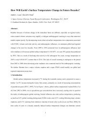
Create successful ePaper yourself
Turn your PDF publications into a flip-book with our unique Google optimized e-Paper software.
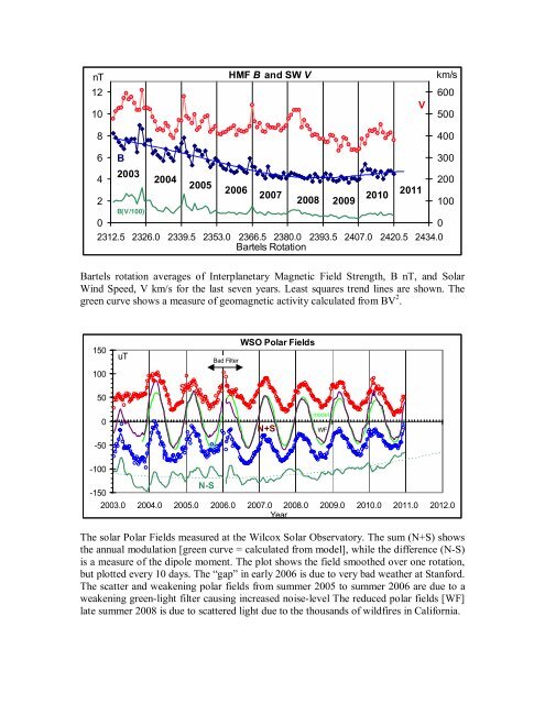
nT12108HMF B and SW VVkm/s6005004006420B2003B(V/100) 230020042002005200620072008 2009 2010 201110002312.5 2326.0 2339.5 2353.0 2366.5 2380.0 2393.5 2407.0 2420.5 2434.0<strong>Bartels</strong> Rotation<strong>Bartels</strong> <strong>rotation</strong> <strong>averages</strong> <strong>of</strong> <strong>Interplanetary</strong> <strong>Magnetic</strong> <strong>Field</strong> <strong>Strength</strong>, B nT, and SolarWind Speed, V km/s for the last seven years. Least squares trend lines are shown. Thegreen curve shows a measure <strong>of</strong> geomagnetic activity calculated from BV 2 .15010050uTSBad FilterWSO Polar <strong>Field</strong>s0N+SmodelWF-50-100-150NN-S2003.0 2004.0 2005.0 2006.0 2007.0 2008.0 2009.0 2010.0 2011.0 2012.0YearThe solar Polar <strong>Field</strong>s measured at the Wilcox Solar Observatory. The sum (N+S) showsthe annual modulation [green curve = calculated from model], while the difference (N-S)is a measure <strong>of</strong> the dipole moment. The plot shows the field smoothed over one <strong>rotation</strong>,but plotted every 10 days. The “gap” in early 2006 is due to very bad weather at Stanford.The scatter and weakening polar fields from summer 2005 to summer 2006 are due to aweakening green-light filter causing increased noise-level The reduced polar fields [WF]late summer 2008 is due to scattered light due to the thousands <strong>of</strong> wildfires in California.
250WSOMWOSolar Mean <strong>Field</strong> Composite (uT)CrAOSOLIS15050-50-150-2502003.0 2003.5 2004.025015050-50-150-2502004.0 2004.5 2005.025015050-50-150-2502005.0 2005.5 2006.025015050-50-150-2502006.0 2006.5 2007.025015050-50-150-2502007.0 2007.5 2008.025015050-50-150-2502008.0 2008.5 2009.025015050-50-150-2502009.0 2009.5 2010.025015050-50-150-2502010.0 2010.5 2011.0a= b=25015050-50-150-2502011.0 2011.5 2012.0
The Mean <strong>Field</strong> <strong>of</strong> the solar disk reduced to the SOLIS scale (which is 1.86 times WSO).The MF is a good proxy for the IMF near the Earth 4.5 days later.Radial component <strong>of</strong> IMF measured by Ulysses spacecraft normalized to distance <strong>of</strong> 1AU. Recent data (dark blue) compared to data from last minimum (red).nT109876543210B obsB calc from IDVB obs median100% =>B std.devCoverage1960 1965 1970 1975 1980 1985 1990 1995 2000 2005 2010109876543210Observed (red) and calculated from IDV (blue) yearly <strong>averages</strong> <strong>of</strong> IMF strength B.-----------Next page: Count <strong>of</strong> ‘active regions with spots’ for the past few cycles. The count isreally a count <strong>of</strong> days in each full month the region was visible [and no more than 70degrees from central meridian] and then summed for every region. Yearly smoothedvalues are also shown as the ‘smoother’ curves. Different cycles are coded with adifferent color. The detailed figures show the transitions between cycles. Note that cycle24 has just barely (but certainly) begun.
500Active Region Count45040035030025020015010050 2122232401980 1985 1990 1995 2000 2005 2010 2015140120100806021 22402001983 1984 1985 1986 1987 1988 198914012010080604022 232001993 1994 1995 1996 1997 1998 19991401201008060402023 2402005 2006 2007 2008 2009 2010 2011 2012
4.0Solar Dipole Divided by Sunspot Number for Following Maximum3.53.02.52.01.51.00.5204521 22 23 24 72165R 240.01965 1970 1975 1980 1985 1990 1995 2000 2005 2010 2015As a measure <strong>of</strong> the solar polar field we take the absolute difference between the Northand South polar fields in the WSO standard 3’ aperture, using MWO averaged into theWSO aperture and scaled to fit WSO [for 1976-1982] before the start <strong>of</strong> the WSOobservations. A ‘polar field cycle’ can be defined from one reversal to the next [roughlyfrom solar maximum to the next solar maximum]. The ‘run’ <strong>of</strong> the polar field values fromeach polar cycle is then divided by the ‘size’ [Rmax] <strong>of</strong> the next sunspot cycle If thepolar fields were controlling Rmax, this procedure would make all the so normalizedpolar cycles look alike. The above plot shows the normalized polar cycles in dark blue.For the latest polar cycle [from 2000 to 2013] we don’t know Rmax for cycle 24, so wedivide by representative guesses [45, light blue; 72, dark blue; 165, pink]. Our prediction[72] would be the divisor that makes the latest polar cycle most like the other ones.------------------------------------15014013012011010090807060F10.7 Radio Flux (@20UT)2005 2006 2007 2008 2009 2010 2011Daily values <strong>of</strong> the F10.7 cm radio flux at 20 UT.
120100ARCActive Region Days (per Month)F10.7Jap.90858080604023 2475702023+24Ri/0.376502007.5 2008 2008.5 2009 2009.5 2010 2010.5 2011 2011.5 201260The number <strong>of</strong> days per month where a NOAA numbered region was on the disk within70 degrees <strong>of</strong> Central Meridian, separately for cycle 23 [blue] and cycle 24 [pink]. Aminimum in December 2008 is suggested. The brown symbols show the F10.7 radio flux[right-hand scale].The data on these pages will be updated about every few weeks.
![When the Heliospheric Current Sheet [Figure 1] - Leif and Vera ...](https://img.yumpu.com/51383897/1/190x245/when-the-heliospheric-current-sheet-figure-1-leif-and-vera-.jpg?quality=85)


![The sum of two COSine waves is equal to [twice] the product of two ...](https://img.yumpu.com/32653111/1/190x245/the-sum-of-two-cosine-waves-is-equal-to-twice-the-product-of-two-.jpg?quality=85)