Analyst Software Reference Guide - AB Sciex

Analyst ® 1.6 SoftwareSoftware Reference GuideRelease Date: August 2011

ContentsSmoothing Algorithms . . . . . . . . . . . . . . . . . . . . . . . . . . . . . . . . . . . . . . . . . . . . .49Software Security . . . . . . . . . . . . . . . . . . . . . . . . . . . . . . . . . . . . . . . . . . . . . . . .49Solvent Compressibility Values . . . . . . . . . . . . . . . . . . . . . . . . . . . . . . . . . . . . . .49Spectral Arithmetic Wizard . . . . . . . . . . . . . . . . . . . . . . . . . . . . . . . . . . . . . . . . .50Spectrum . . . . . . . . . . . . . . . . . . . . . . . . . . . . . . . . . . . . . . . . . . . . . . . . . . . . . . .50Syringe Size Versus Flow Rate . . . . . . . . . . . . . . . . . . . . . . . . . . . . . . . . . . . . . .50Weighting Factors . . . . . . . . . . . . . . . . . . . . . . . . . . . . . . . . . . . . . . . . . . . . . . . .52Chapter 2 PPG Exact Mass Table. . . . . . . . . . . . . . . . . . . . . . . . . . . . . . . . . . . . . 534 Release Date: August 2011

ForewordThis software reference guide provides information about the Analyst ® software features.Related DocumentationThe guides and tutorials for the instrument and the Analyst software are installed automaticallywith the software and are available from the Start menu: All Programs > AB SCIEX > Analyst. Acomplete list of the available documentation can be found in the online Help. To view the Analystsoftware Help, press F1.Technical SupportAB SCIEX and its representatives maintain a staff of fully-trained service and technicalspecialists located throughout the world. They can answer questions about the instrument or anytechnical issues that may arise. For more information, visit the Web site at www.absciex.com.Release Date: August 2011 5

Foreword6 Release Date: August 2011

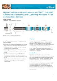
Terms and Concepts1Analyst Software ModesThe software is divided into modes, which are discrete functional areas you can perform a rangeof activities related to a main task. You can access modes through the Navigation Bar or theMode list in the toolbar and can switch from one mode to another without losing any work. Formore information, see the Analyst ® software Show Me tutorial.12Figure 1-1 Analyst Software WindowItem Description1 Mode list2 Navigation BarAnalyst Software FeaturesAs well as the main features of acquisition and processing, the software has some features thathelp you run your experiments more efficiently and more quickly.Release Date: August 2011 7

Terms and ConceptsIDAIDA (Information Dependent Acquisition) is an acquisition method that analyzes data duringacquisition. You can use IDA to change the experimental conditions depending on the analysisresults. These real-time changes are controlled by criteria set in the acquisition method,including:• Ion intensity and charge state.• Inclusion and exclusion lists.• Isotope pattern.Being able to optimize data acquisition settings while the data is being acquired enables you toconserve both the sample and working time on an instrument.Queue ManagerThe Queue Manager shows queue, batch, and sample status and lets you manage samples inthe queue.Library SearchLibrary Search lets you create and manage a mass spectra database by helping you to searchfor and match unknown spectra against the mass spectra stored in the database.Fragment Interpretation ToolThe Fragment Interpretation tool helps you interpret MS/MS data. Given the chemical structure ofa molecule, this tool can generate a list of theoretical fragment masses from single non-cyclicbond cleavage of that molecular structure. The tool can then match the theoretical list with peaksin the current mass spectrum.Express ViewUse Express View when you want to create a batch quickly or when you need to add a samplename or change a small number of fields to an existing template. It provides a simplified interfacefor sample submission, while restricting further access to other functions. To use Express View,you select a batch template, type user information, and then submit a batch.WorkspacesA workspace is a particular arrangement of windows and panes, including any associated file orfiles. For example, while working on a particular data set, you have opened and sized variouswindows to help you with your analysis. You can save this arrangement, or workspace, so thatthe next time you look at the data, the window arrangement is identical.In Quantitate and Explore modes, you can have multiple workspaces per session. This meansthat you can design different workspaces to suit different tasks within these modes, and thensave them for future use. When in one of these two modes, you can open a particular workspacewithout exiting that mode.8 Release Date: August 2011

Software Reference GuideAnalyst ServiceThe Analyst Service is the communication path between the mass spectrometer and attachedperipheral devices.The service is started each time you launch the Analyst ® software. In general, however, theAnalyst Service starts automatically when you log on to Windows. If for any reason the service isnot running when you try to start the Analyst software, perhaps there was a problem starting theservice at the time of log on, or if it was manually stopped, the Analyst Service will start up at thattime. For this reason, starting or restarting the Analyst Service is almost always doneautomatically.API Instrument Project FoldersThe following are some of the folders found in the API Instrument project.• API BioAnalyst: Contains the BTB Data Dictionary.csv file, the file containing thedefault Data Dictionary information required for the BioAnalyst software. Theappropriate folders appear only when the BioAnalyst software is installed.• Bundler: Contains a program that takes all aspects of a .wiff file and automaticallycombines them when the sample is completed.• Configuration: Contains all the hardware profiles (.hwpf files).• Example Scripts: Contains some of the scripts that are used throughout thesoftware.• Instrument Data: Contains a file called InstrumentData.ins, which stores all thecritical calibration information and more.• Method Tables: Contains all instrument settings that define the enhanced scanfunctions. Do not change the files in this folder. Changing the contents of this folderwill affect the performance of the enhanced scan modes.• Parameter Settings: Contains all the instrument settings and linkages. Instrumentsettings are saved as ParamSettingsdef.psf files.• Preferences: Contains the Tunedata.tun file. All settings (parameter, tuning,instrument, processing, appearances and queue) are saved as Tunedata.tun in thisfolder.• Processing Scripts: Contains the scripts for data processing in Explore mode. Theyare found in the Script menu in the Analyst software.• Queue Data: Contains information from the queue.• Tuning Cache: Contains all the data created in Manual Tuning by clicking Startinstead of Acquire. Files are saved with a generic time and date stamp for theirnames. The tuning cache holds a limited number of files and will overwrite files asneeded. Rename and move the files immediately if they need to be saved.Area Threshold ParametersSee Noise and Area Threshold Parameters on page 25.Release Date: August 2011 9

Terms and ConceptsAutotune Instrument Optimization AlgorithmThe Autotune Instrument Optimization algorithm tunes both quadrupole and LIT modes andperforms mass calibration. For quadrupole mode, it adjusts the resolution offsets. For LIT mode,it optimizes AF3 and EXB. For MS3, it adjusts the excitation and isolation coefficients.Background SubtractBackground subtract reduces the amount of noise in a spectrum by subtracting either one or tworanges that contain noise from a range that contains a peak. You can move the rangesindependently or lock them and move them as a single entity within the graph. LockedBackground Subtract is the preset setting.You can use background subtraction to isolate a peak of interest. You can highlight and subtractup to two selected ranges from your peak. You can also lock your ranges and move them withinthe graph to optimize peak isolation or to isolate another peak.Background Subtract to FileYou can use Background Subtract to File to save a new file that has a defined noise regionsubtracted from each scan. When a range is selected in the TIC, all the scans from that selectionare internally averaged, and the resulting spectrum is subtracted from all the scans. Use theBackground Subtract to File dialog to select where the file is to be saved. You also have theoption of naming the new file. In some cases, the resulting file might look close to the originalscanBaseline SubtractBaseline subtract removes a constant or slowly varying offset from a set of data. This is useful inlocating small peaks that are obscured by noise. The software uses the following algorithm inperforming a baseline subtraction.1. Every data point in the data set is considered as the center of a window (in mass ortime) with a user-definable width measured in amu or minutes.2. The minimum values on either side of the current data point (minima) within thewindow are located.3. A straight line is fitted between the two minima and the height (intensity) of thecurrent data point above the line is calculated. The end points of the data areregarded as minima.4. The data point is replaced with the new calculated value.BatchesA batch is a collection of information about the samples that you want to analyze. Samples areusually grouped into sets to make it easier for you to submit them. Grouping your samples into aset also reduces the amount of data you must manually enter. A set can consist of a single10 Release Date: August 2011

Software Reference Guidesample or multiple samples. All of the sets in a batch use the same hardware profile; however,samples in a set can have different acquisition methods. A batch can be submitted only from anacquisition station.Batches link together:• Sample information, such as name, ID, and comment.• Autosampler location (rack information).• Acquisition methods.• Processing method or script (optional).• Quantitation information (optional).• Custom sample data (optional).• Set information.Batch EditorThe Batch Editor is used for creating and modifying batches and for creating batch templates. Torun samples, each using different acquisition methods, use the Batch Editor to select multipleacquisition methods in the same set. In the Batch Editor, you can also use an acquisition methodas a template. In this case, the same method is used for each sample, but you can selectdifferent masses or mass ranges for each sample.You can also modify every detail of the batch before submitting it for processing. When yousubmit a batch for analysis, you can submit the entire batch, specific sets within the batch, orspecific samples within a set.For example, you may want to analyze ten samples, five using one acquisition method and fiveusing a different acquisition method. You could create a batch of two sets, one for each methodthat you want to use.You can also use the Batch Editor to import sample lists created in external programs, such asMicrosoft Excel. The Batch Editor has the following tabs:Table 1-1 Batch Editor TabsTabSampleLocationsQuantitationSubmitDescriptionUsed to create the sample list and to select sample details such as the samplename and the acquisition method to be used to acquire the sample.Used to select the positions of samples in the autosampler. Sample locationscan be specified numerically in the Sample tab; however, the Locations tabprovides a graphical interface for selecting sample locations.Used to select the sample types and concentrations for quantitation batches.Because quantitation information can be specified post-acquisition in thequantitation Results Table, you do not have to use the Quantitation tab in theBatch Editor. Instead, you can use the Quantitation Wizard.Used to verify sample information and to submit samples to the acquisitionqueue.Release Date: August 2011 11

Terms and ConceptsAbout Importing Batch FilesTo make data entry easier, you can import batch file information from other applications. TheBatch Editor can import text and other files that are formatted correctly. For examples of correctlyformatted files, refer to the Batch folder in the Example project.The information in a batch file can also be exported for use with other applications, such asMicrosoft Excel, Microsoft Access, and certain LIMS (Laboratory Information ManagementSystem) software.CalculatorsWith the Calculator window, you can perform calculations on the basis of collected data.Although the calculator is a separate window, it is connected to the active graph within thesoftware.The following calculators are available.• Elemental Composition Calculator• Hypermass Calculator• Elemental Targeting Calculator• Mass Property Calculator• Isotopic Distribution CalculatorYou can cut and paste from one text box to another between the different windows in thecalculators. You can also print data from any of the calculators by clicking the Print icon in the topleft corner of the window. For more information about using calculators, see the Help.Data from the Elemental Composition, Mass Property, and Isotopic Distribution calculators canbe exported to a separate file. Use the Elemental Targeting calculator to modify the data withinthe active graph. Data from the HyperMass and Isotopic Distribution calculators can be overlaidon the active spectrum.Tip! You can set the precision of calculator data in the Calculators tab of theAppearance Options dialog. To open the dialog, click Tools > Settings > AppearanceOptions.Elemental Composition CalculatorThe Elemental Composition calculator determines potential molecular or amino acidcompositions based on a target mass-to-charge ratio. You can type this ratio manually or select itfrom an active spectrum. This calculator creates a table with the possible element or amino acidcombinations making up the mass of interest and the characteristics of each.You can type or select values for such parameters as tolerance, electron state, and number ofcharges. You can also type a list of possible elements and put a limit on the number of each.Hypermass CalculatorThe Hypermass calculator determines the distribution of a multiply charged envelope based onan uncharged mass. You can select the uncharged mass, including the adduct and its polarity.12 Release Date: August 2011

Software Reference GuideThe calculator displays a graphical representation of the Hypermass series, which can beoverlaid onto the active spectrum. A list of the Hypermass data is also available.Elemental Targeting CalculatorThe Elemental Targeting calculator reduces the data spectrum based on a specific pattern,primarily one corresponding to isotopic distributions. It can also search an MS data spectrum fora specific pattern of peaks, which can be entered either as a formula or as an isotopicdistribution.If the calculator finds a match, it creates a reduced plot containing only data pertaining to thespecified pattern. For a spectrum, the calculator removes all unmatched data. For achromatogram, the calculator calculates the elemental target for each of the underlying spectraand regenerates each point in the chromatogram on the basis of these new spectra.Mass Property CalculatorThe Mass Property calculator determines various properties such as exact mass, the averagemass, the mass accuracy, and the mass defect of a mass of interest. The results generated bythis calculator depend upon the number of input fields completed.Isotopic Distribution CalculatorThe Isotopic Distribution calculator determines the isotopic distribution based on an enteredformula. This allows you to distinguish between compounds with the same mass based onrelative intensities of isotopes.The calculated isotopic distribution can be displayed in graphical or text format on the IsotopicDistribution pane, overlaid on the active spectrum, or exported to a separate file.Calibration OptionsThe calibration options define the parameters for a calibration curve, which are used todetermine the calculated concentration of the samples. The curve is a plot of the concentration ofthe standard against the area or height of the standard if no internal standard is used. If aninternal standard is used, the curve is a plot of the concentration ratio against the area or heightratio. This curve is used, along with the area (or height) for the unknowns, to interpolate thecalculated concentration.You must choose the best regression type or fit to fit the curve to the points and the bestweighting factor for your project.About Calibration CurvesThe calibration curve is used to determine the calculated concentration of samples, including QCsamples. It is a curve that results from plotting the concentration of the standard versus its areaor height, or ratios, if you are using an internal standard. The area or height of a sample is thenapplied to this curve to determine the sample concentration, as displayed in the Results Table.The regression equation generated by this calibration curve is used to calculate theconcentration of the unknown samples.Release Date: August 2011 13

Terms and ConceptsThe software places the known concentrations (or ratios) on the x-axis and the calculated area orheight (or ratios) on the y-axis. It then plots the points for all the standards in the batch. Thesystem produces a best-fit curve to those points through regression and weighting type that youchoose. This curve is used, along with the area (or height), for the unknowns to interpolate theconcentration.Selecting the Best Regression TypeAfter you select a regression type (fit), you cannot see the calibration curve from the wizard.Instead, you may use the preset values, rely on your experience, or use your corporate policy tochoose a regression type.After you change the fit, check the Accuracy column in the Results Table for changes. You willfind that the better the fit is, the better the accuracy of the quantitative analysis will be.The calibration curve plots the standards concentration against its peak area or height (or ratios,if an internal standard is used). When the points for the standards are plotted, determine the bestfit for the curve to these points and indicate your choice in the Specify Calibration dialog of thewizard. The preset fit is linear, which assumes that all your standards will fall on a straight line.Select from the types of fit in Table 1-2.Table 1-2 Types of FitFitLinearLinear Through ZeroQuadraticMean Response FactorPowerChoosing the Best Weighting FactorDescriptionLinear regression assumes that the standard points fall on a straightline.Linear Through Zero regression assumes that the standard points fallon a straight line and that the points line up with the zero point on thex- and y- axes. Use this setting to force the line to go through the zeropoint.If the standard points do not fall on a straight line, use quadraticregression to produce a quadratic fit to the data points.If the standard points fall on a straight line and you want to averagethe points, use mean response factor regression to produce anaverage of the slope for every point on the curve.If there is some linear and some curvature in the line of points, usepower regression instead of linear or quadratic regression to producea line somewhere between these fits.The calibration curve plots the standards concentration against its peak area or height. When thepoints for the standards are plotted, you must determine the best weighting factor for these pointsand indicate your choice in the Specify Calibration dialog. The default fit is None, which assumesthat all points along the curve have the same importance. Select from the types of weighting inTable 1-3.Table 1-3 Types of WeightingWeighting Description1/x To place some additional emphasis on lower-value points, use a weightingfactor of 1/x.14 Release Date: August 2011

Software Reference GuideTable 1-3 Types of Weighting (Continued)WeightingDescription1/(an)Use a weighting of 1/x 2 to place much higher emphasis on lower-valuepoints.1/y Use a weighting factor of 1/y when you are calibrating by the area (y-axis)rather than by the concentration (x-axis), and you want to place someemphasis on lower-value points. A weighting of 1/y is a variant of 1/x where yand x should be proportional to each other.1/(y*y)Use a weighting factor of 1/y 2 when calibrating by the area (y-axis) ratherthan by the Concentration (x-axis), and you want to place much higheremphasis on lower-value points. A weighting of 1/y squared is a variant of 1/x squared where y and x should be proportional to each other.In xUse the logarithm of x to place more emphasis on higher-value points.In yUse the logarithm of y to place more weight on higher-value points. Usewhen calibrating by the area (y-axis) rather than by the concentration (xaxis).ChromatogramsA chromatogram displays the variation of some quantity with respect to time in a repetitiveexperiment; for example, when the instrument is programmed to repeat a given set of massspectral scans several times. Chromatographic data is contiguous, even if the intensity of thedata is zero. Chromatograms are not generated directly by the instrument, but are generatedfrom mass spectra.In the chromatogram display, the intensity, in counts per second (cps), is shown on the y-axisversus time on the x-axis. Peaks are automatically labeled.In the case of LC/MS, the chromatogram is often displayed as a function of time, the time atwhich a particular scan was obtained, which can be derived from the scan number.Compound DatabaseThe compound database stores information about compounds, including optimizationspecifications.Use the compound database when you have large numbers of samples and need to optimize alarge number of compounds quickly. The Automaton software automatically fills the database.The Compound Database window stores optimized conditions for compounds that can beretrieved to run samples.Compound OptimizationThe Compound Optimization software wizard automatically optimizes an analyte. You canintroduce the sample using infusion or FIA (flow injection analysis.) The software first checks forthe presence of the compounds. The voltages of the various ion path parameters are graduallyincreased or decreased to determine the maximum signal intensity (Q1 scan) for each ion. A textRelease Date: August 2011 15

Terms and Conceptsfile is generated and displayed during the optimization process. This file records the variousexperiments performed and the optimal values for each ion optic parameter. A file foldercontaining all the experiments performed is also generated and can be found by opening the datafile folder in Explore mode. For each experiment performed, an acquisition method is alsogenerated and saved in the acquisition method folder.See also Flow Injection Analysis (FIA) on page 17 and Infusion on page 19.Dynamic Background Subtraction AlgorithmDynamic Background Subtraction algorithm improves detection of precursor ions in an IDA(Information Dependant Acquisition) experiment. When the algorithm is activated, IDA uses aspectrum that has been background subtracted to select the ion of interest for MS/MS analysis,as opposed to selecting the precursor from the survey spectrum directly. Because this processtakes place during LC analysis, the algorithm enables detection of species as their signalincreases in intensity, therefore focusing on detection and analysis of the precursor ions on therising portion of the LC peak, up to the top of the LC peaks (maximum intensity).Dynamic Fill TimeDynamic Fill Time (DFT) is a feature specifically designed to optimize the data obtained in everyspectrum for the linear ion trap scan functions. DFT will automatically adjust the fill time used tofill the ion trap based on the ion flux coming from the source. For more intense ions, the fill timewill be automatically reduced to ensure the trap is not overfilled with ions.For less intense ions, the fill time will be automatically increased, ensuring that good ion statisticsare obtained in the spectrum. DFT is applicable for the following scan types:• Enhanced MS (EMS)• Enhanced Resolution (ER)• Enhanced Product Ion Scan (EPI)• MS/MS/MS (MS3)You can adjust the DFT settings by selecting Tools > Settings > Method Options in the Analystsoftware.Experiments and PeriodsThe mass spectrometer acquisition method consists of experiments and periods. In theAcquisition Method Browser pane, you can create a sequence of acquisition periods andexperiments for the mass spectrometer. You can also open a method previously created in theTune Method Editor.ExperimentsAn experiment includes the mass spectrometer settings and scan type during an MS scan. A setof MS scans performed for a specific amount of time is called a period. An acquisition method inwhich the MS parameters and actions are the same through the entire duration is called a singleperiod,single-experiment method.16 Release Date: August 2011

Software Reference GuideIn looped experiments, MS settings are changed on a scan-by-scan basis. For example, if thesample contains two compounds, A and B, you may want to loop an MS/MS experiment ofcompound A with an MS/MS experiment of compound B to obtain information on bothcompounds in the same run. The mass spectrometer method will alternate between the twoscans. Other examples of looped experiments include alternating between positive and negativemode in a run and IDA methods.PeriodsA period can contain one or more looped experiments. In a multi-period acquisition method,experiments are performed for a specified amount of time and then switch to another set ofexperiments. Periods are useful when you know the elution time of the compounds in an LC run.You can have the mass spectrometer perform different experiments according to when thecompounds elute to get as much information as possible in the same run.In Figure 1-2, a three-period method is shown. The first period has a duration of 3.015 minutes;the second period is 4.986 minutes; and the third period is 7.000 minutes.Figure 1-2 Example of a multi-period experimentFlow Injection Analysis (FIA)FIA is the injection of a small quantity of a sample by an autosampler into the LC stream. Duringthe FIA optimization process, multiple sample injections are performed for various source- orcompound-dependent, or both, parameter types that are changed between injections. FIAoptimizes for declustering potential, collision energy, and collision cell exit potential by performinglooped experiments in succession, that is, one compound-dependent parameter followed by thennext compound-dependent parameter. It optimizes for source-dependant parameters by makingan injection for each parameter.Use FIA optimization to optimize both compound- and source-dependent parameters using LC athigher flow rates. See also Infusion on page 19.Release Date: August 2011 17

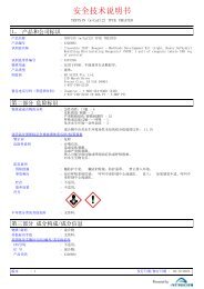
Terms and ConceptsIDA ExplorerThe IDA (Information Dependent Acquisition) Explorer is used to display data acquired throughan IDA method.The IDA Explorer can be turned off and on by going to the IDA Explorer tab in the AppearanceOptions dialog. Columns present in the List View can be defined under this tab as well.The left side of the viewer shown in Figure 1-3 displays the masses on which a product ion scanwas performed. In this area, you can examine the mass, intensity, time, and collision energy ofions on which product ion scans were performed. You can view these in either a list view or a treeview. In list view, the list can be sorted by double-clicking on any column header. In theAppearance Options dialog, you can customize the columns you want to view in the list view.On the right side, the viewer is split into four panes. The top left pane displays the survey TICdata. The bottom left pane shows the XIC of the mass. The top and bottom right panes show thesurvey and product scans, respectively.The IDA viewer lists all the masses on which Enhanced Product Ion scans or EnhancedResolution scans were performed. Click a mass in the list or tree view to display plots relevant tothat mass. You can view the survey spectrum from which the mass was identified and the productspectrum of that mass. It also displays the TIC of the survey scan and the XIC for each mass.Note: Brackets around a mass indicate that the mass is merged. A merged mass iscontiguous across a number of cycles. When a merged mass is displayed, it indicatesan averaged spectrum, containing the average of all contiguous spectra.Figure 1-3 IDA Viewer18 Release Date: August 2011

Software Reference GuideIDA MethodsAn IDA (Information Dependent Acquisition) method automatically runs experiments based onresults obtained from previous experiments. Use IDA criteria to optimize data acquisition settingswhile acquiring data to reduce the sample acquisition time in a single injection. With IDA, you canconserve both the sample amount required and working time.Create an IDA method with up to two survey scans and eight dependent scans in a singleexperiment. A survey scan is used in IDA to trigger additional experiments. You can use thefollowing scans as a survey scan:• Enhanced Multiply-Charged (EMC).• Enhanced Product Ion (EPI) (second survey scan).• Enhanced MS (EMS).• MRM.• Neutral Loss (NL).• Precursor Ion (Prec).• Q3 MS.You can use the following dependent scans:• EPI.• MS/MS.In an IDA experiment, the mass spectrometer actions are varied from scan to scan based on thedata acquired in a previous scan. The software analyzes data as it is being acquired and thendetermines the masses on which to perform dependent scans. You can set the criteria that willactivate an IDA experiment and the method parameters to be used.IDA experiments modify experiments and improve results based on the following user-definedcriteria:• Ion intensity and charge state.• Inclusion and exclusion lists.• Isotope pattern.• Dynamic exclusion.• Rate of change in ion intensity (See Dynamic Background Subtraction Algorithmon page 16).InfusionInfusion is the continuous flow of the sample at low flow rates into the ion source using a syringepump. During the infusion optimization process, the software can select precursor and productions and optimize for declustering potential, collision energy, and collision cell exit potential forboth. The voltages of these ion path parameters are gradually increased or decreased todetermine the maximum signal intensity for the precursor and product ions.Use infusion optimization to optimize compound-dependent parameters only at much lower flowrates than those used during LC/MS analysis. See also Flow Injection Analysis (FIA) on page 17.Release Date: August 2011 19

Terms and ConceptsIntegration AlgorithmsThe Analyst ® software has two integration algorithms: the original Analyst Classic integrationalgorithm and the IntelliQuan integration algorithms. The IntelliQuan algorithm provides moreconsistent peak-finding and integrated functionality, with fewer parameters that requireadjustment.Analyst Classic and IntelliQuan Integration AlgorithmsThe IntelliQuan algorithm uses one of two peak-finding parameters: Automatic IQA II, which is aparameterless setting, or Specify Parameters MQ III. After integrating peaks using the IntelliQuanalgorithm, you can choose which peak-finding parameter best fits the data set. This is done in thedisplayed peak integration parameters in the Peak Review pane or window.Table 1-4 shows the parameters available with the Analyst Classic algorithm.Table 1-4 Analyst Classic AlgorithmParameterDefault Bunching FactorDefault Number of SmoothsDefault Void Volume RetentionTimeDefault Concentration UnitsDefault Calculated ConcentrationUnitsDefault RT WindowDefinitionThe number of points to be averaged together andconsidered as a single point for the purpose of peak-finding.The number of times to smooth the chromatogram.Any peaks that appear before this time are ignored.The concentration units used to describe the sampleconcentration, for example, pg/µL.The concentration units used to describe the calculatedsample concentration, for example, pg/µL.The time window centered at the expected retention time forpeak-finding. For example, a 30 second retention timewindow gives an additional 15 seconds before and after theexpected retention time.Table 1-5 shows the parameters available with the MQ III algorithm, but not the IQA II algorithm.Table 1-5 MQ III AlgorithmParameterDefault Noise PercentageDefault Baseline SubtractionWindowDefinitionThe threshold used in peak-finding. Only peaks higher thanthis specified percentage will be detected.A time window around each data point that is used todetermine the height of the baseline correction to be appliedto that point. This time window helps remove excessivenoise from the chromatogram. The baseline is defined asthe line connecting the point of minimum intensity on the leftside of a given data point to the point of minimum intensityon the right side, within the specified window.20 Release Date: August 2011

Software Reference GuideTable 1-5 MQ III Algorithm (Continued)ParameterDefault Peak-Splitting FactorDefault Void Volume RetentionTimeReport Largest PeakDefinitionControls whether a given peak cluster consists of multipleadjacent peaks or one (possibly noisy) peak. If the intensitydip is less than the value specified, then a single peak isreported; otherwise the point with minimum intensity in thedip splits the cluster into two separate peaks. Setting a largefactor will prevent clusters from being split into more thanone peak.Any peaks that appear before this time are ignored.Selecting this parameter returns the largest peak in theretention time window. If this parameter is not selected, theclosest peak to the expected retention time is found. Theexpected retention time is automatically calculated in theQuantitation Wizard.Table 1-6 shows the parameters available for use with both IntelliQuan algorithms.Table 1-6 IntelliQuan AlgorithmParameterDefault Minimum Peak HeightDefault Minimum Peak WidthDefault RT WindowDefault Smoothing WidthDefault Concentration UnitsDefault Calculated ConcentrationUnitsDefinitionThe minimum height of a peak required for peak integration.The minimum width of a peak required for peak integration.Specifies the time window centered at the expectedretention time for peak-finding. For example, a 30 secondretention time window gives an additional 15 seconds beforeand after the expected retention time.The number of points used in data smoothing.The concentration units used to describe the sampleconcentration, for example, pg/µL.The concentration units used to describe the calculatedsample concentration, for example, pg/µL.Interface Heater Temperature (IHT)The IHT parameter controls the temperature of the NanoSpray ® ion source interface heater. Theoptimal heater temperature depends on the type of sample you are analyzing and the solventused. If the heater temperature is too high, the signal degrades. The maximum heatertemperature you can set is 250 °C, but this is too high for most applications. Typically, heatertemperatures are in the 130 to 180 °C range.LC MethodsIf you are creating a new acquisition method file from an existing file, you may decide to usesome or all of the device methods in the acquisition method. With the Acquisition Method Editor,Release Date: August 2011 21

Terms and Conceptsyou can customize the acquisition method by adding or removing HPLC peripheral devicemethods.You can create an acquisition method for an HPLC peripheral device means by selecting theoperating parameters for that peripheral device. Methods can be created for any of the followingperipheral devices if they are configured in the active hardware profile:• Pumps.• Autosamplers.• Syringe pumps.• Column ovens.• Switching valves.• Diode array detector.• Analog-to-digital converters.• Integrated systems.For information about setting properties for peripheral devices, see the Peripheral Devices SetupGuide.Library DatabasesThe Library Search feature compares unknown spectra to known MS spectra contained in alibrary database and generates a list of possible matches.With Library Search you can:• Compare library contents against an unknown spectrum.• Add records to the library.• Edit existing records.You can store library data in the following locations:• MS Access on a local database.• MS SQL Server.Before you can use the Library Search feature, determine where the library database is storedand connect your computer to that location. Library databases can be stored locally and over anetwork.To connect to a database, use an alias. In this case, the alias specifies a connection to a specificdatabase and may include the user name and password required to access the database. Forexample, you may have a small library database of your own identified compounds on yourcomputer and your organization may have a central database that you use occasionally. Creatingaliases for each database allows you to switch between them quickly. For information aboutcreating aliases and connecting to databases, see the Help.Method-Creation ToolsThe software offers four quantitation method-creation tools, each of which creates a fullyfunctional method. The best choice of tool depends on the tasks you need to accomplish.22 Release Date: August 2011

Software Reference GuideWizardsThere are two available method-creation wizards: the Standard Quantitation wizard and theAutomatic Quantitation wizard. Both allow you to select the batch or batches to be quantified,create or select a quantitation method, and then integrate the sample data.The difference between the two is the type of method you create. The standard wizard creates astandard method, while the automatic wizard creating methods. You do not verify the peaks aspart of the method creation (you can still review the peaks after integration has taken place).There is only one common occasion for which you would not need to verify the peaks: when youare doing quantitation simply to integrate, not to find concentrations. You might want to do this,for example, if you have a batch that contains different compounds in every sample, or when themass is not the same from sample to sample. If this is the case, use the automatic wizard.Otherwise, to perform quantitation, use the standard wizard.Use the Standard Quantitation wizard after you have acquired your sample and you want to:• Choose a representative sample.• Select analyte and internal standard peaks.• Adjust peak-finding and integration parameters.• Review peaks during method creation.• Select calibration.Use the Automatic Quantitation wizard to select a batch, create a method (without peakconfirmation), and then integrate the sample data. This wizard is quicker than the Standardwizard and does not require that the masses scanned be the same for all samples. It does not,however, allow you to select an internal standard—all ions are treated as analytes.Use the Automatic Quantitation wizard after you have acquired your sample and you:• Want to select calibration.• Do not want to adjust peak-finding and integration parameters.• Do not want to select analyte peak names.• Do not want any internal standards.• Do not want to review peaks during method creation, or you have differentcompounds in every sample.When you are only integrating peaks, you do not need to verify them as no concentrationcalculation is required. In this case, use the Automatic quantitation method creation, which allowsyou to review the peaks after integration has taken place.Finding Peaks Using an Automatic MethodThe software uses the standard peak-detection process, with the following exceptions:• It uses the bunching factor and the number of smooths (from the wizard) as is.• It calculates the expected retention time and noise and area thresholds separatelyfor every peak.Release Date: August 2011 23

Terms and ConceptsQuantitation Method EditorUse this option after you have acquired your sample and you want to:• Adjust peak-finding and integration parameters.• Select analyte and internal standard peaks.• Select calibration.You can use the Quantitation Method Editor to do three additional tasks:• Sum ions for integration.• Use an internal standard from a different period or experiment (if the internalstandard was acquired in a different period or experiment than the analyte).• Edit an existing method.The Semi-Automatic Method EditorThe Semi-Automatic Quantitation Method Editor is part of the Batch Editor. You can use theSemi-Automatic Quantitation Method Editor to select quantitation information, such as sampletype and sample concentration, prior to data acquisition. This preparation makes performingsubsequent quantitative analysis easier. Alternatively, you can select a full method in the BatchEditor, which is then automatically applied at the end of the batch run to generate the quantitationResults Table.Use this option when you:• Have not yet acquired any samples.• Want to select names and masses for analyte and internal standard peaks.• Want to select concentrations and sample types on the Quantitation tab in the BatchEditor, but do not have any other quantitation method.• Want to edit the quantitation method, if necessary, at a later time.Finding Peaks Using a Semi-Automatic MethodThe software uses the standard peak-detection process, with the following exceptions:• It uses the bunching factor (from the Quantitation Method Options dialog) and thenumber of smooths (from the Create Semi-Automatic Quantitation Method dialog) asis.• It uses the most concentrated standard as the representative sample. To establish aretention time, it uses the largest peak within that chromatogram.• To set noise and area thresholds, it uses the resulting baseline noise. (This processis identical to how the default values are set for peaks in normal methods.) Theseintegration parameters are applied to all other samples.• If the batch being examined does not contain quantitation information (sample typeand concentrations), the retention time and thresholds are calculated separately forevery peak (as for fully automatic methods).24 Release Date: August 2011

Software Reference GuideNoise and Area Threshold ParametersTo identify peaks, the software requires a set of noise and area threshold parameters. Thesoftware sets these parameters initially, but you can change them later. It sets the parameters asfollows:1. The software calculates the largest intensity difference between any two sequentialdata points. This number represents the difference between two intensities, not theactual intensity itself.2. For each sequential pair with an intensity difference of less than 5% of the valuecalculated in Step 1, it calculates the standard deviation (using a mean of zero) ofthe intensity differences. (The software does not use those pairs of points with anintensity difference larger than 5% of the maximum.)It sets the noise and area thresholds as follows:3. The noise threshold is equal to the standard deviation calculated in step 4.4. The area threshold is equal to five times the noise threshold.Note: The minimum value for both the noise and area thresholds is 0.000001. If thecalculations produce a value that is lower than this minimum, then the software resetsthe value of that threshold at 0.000001.Recalculating the Noise and Area ThresholdIf you define a new background area, the software recalculates the noise and area thresholds asfollows. For each sequential pair of data points, the software calculates the standard deviation,using a mean of zero, of the intensity difference. The Analyst software uses all points within theselected range because you are explicitly telling it that the selected area is background noise.It sets the noise and area thresholds as follows:1. The noise threshold is equal to the standard deviation calculated for the selectedrange.2. The area threshold is equal to five times the noise threshold.Note: The minimum value for both the noise and area thresholds is 0.000001. If thecalculations produce a value that is lower than this minimum, then the software resetsthe value of that threshold at 0.000001.Peak IntegrationThe following are integration types by which the baseline was found and integrated when thepeak was found.• Manual: The peak was manually integrated by the user.• Automatic: The peak was automatically integrated as follows:• Baseline-to-baseline: The peak area is defined by vertical droplines at thebeginning and end of the peak which extend to the baseline. This integrationtype is possible only for peaks that do not have another peak immediatelypreceding or following.Release Date: August 2011 25

Terms and ConceptsPeak Review• Valley: Same as baseline-to-baseline, except that it applies only to peaks thatdo have another peak immediately preceding or following.• Exponential Skim: The peak area is the main or parent peak in anexponential skim.• Exponential Child: The peak area is the child peak resulting in anexponential skim.During peak review you can survey the peaks that the software selected and then redefine thepeak or the start and end points where necessary.Reviewing PeaksIn general, the software is adept at accurately identifying analyte and internal standard peaks.For a variety of reasons, including sample acquisition and quantitation method definition,sometimes the software misses the correct peak, chooses the wrong one, or is unable to locate apeak at all. Other times, although the software may correctly identify the peak, you might notagree with the start or end points selected.Detecting PeaksThe software detects peaks in four stages.1. First, it finds the potential peak start by examining the distance between eachbunched point and the preceding one. When the distance exceeds the current noisethreshold, a potential peak start has been found.2. Then it confirms the peak start by making sure that enough points exist in a row toexceed the area threshold.3. Next, it finds the peak top by searching for a point that is lower than the previouspoint.4. Finally, it finds the end of the peak by identifying the place where the distancebetween one bunched point and the next falls below the noise threshold. Ifnecessary, it then separates peaks.26 Release Date: August 2011

Software Reference GuideFinding the Potential Peak StartTo find the potential start of a peak, the software measures the intensity difference betweensequential pairs of bunched points, starting at the first point. When it finds a difference thatexceeds the current noise threshold, the software declares the first point a potential peak start.123Figure 1-4 Finding the potential peak startItem Description1 Exceeds noise threshold2 Potential peak start3 Does not exceed noise thresholdConfirming the Peak StartTo make sure that it has found a real peak, the software moves along the curve, adding theintensity difference between each bunched data point from the intensity at the potential peak startto a total sum. This process stops when the intensity difference between successive points is lessthan the noise threshold. This sum is an approximation of the area of the leading edge of thepeak. If this sum exceeds the area threshold, then the software confirms the peak start.Next, the software determines the actual start of the peak by moving backward from the potentialpeak start until it finds the lowest point in the peak. It moves back through five bunches of rawdata. This point is the actual peak start.Release Date: August 2011 27

Terms and Concepts1Figure 1-5 Confirming the peak startItem Description1 Sum of area slices greater than threshold13Figure 1-6 Confirming the actual peak startItem Description1 Look through data points in this region2 Minimum data point3 Potential peak startFinding the Peak Top2To find the peak top, the software first looks for a point that is lower than the preceding point.Then, to confirm that it has found the top correctly, it sums the intensity differences between thepotential top and subsequent bunched points until it reaches the end of the peak. If the totaldistance between points exceeds two-thirds of the area threshold, then the peak top isconfirmed. That is, the software makes sure it has a peak first, and then works backward to findthe top of it.28 Release Date: August 2011

Software Reference GuideIf, however, the software finds a higher bunched point before the area test has been passed, thenit identifies a new top and restarts the area test.Note: The actual retention time for a peak is not simply the point identified asdescribed previously. Instead, it is determined from a quadratic fit based on the threehighest data points.1Figure 1-7 Finding the peak topItem Description1 Sum of area slices is greater than two thirds of the area threshold1Figure 1-8 Identifying a new peak topItem Description1 The shoulder has a maximum, but the cumulative crest area is not greater than twothirds of the area thresholdRelease Date: August 2011 29

Terms and ConceptsFinding the Peak EndThe software declares a peak end point when one of the following occurs:• The difference between two consecutive points fails the noise threshold test.• The software detects the start of a new peak.In either case, the lowest bunched point from the last five bunches is considered to be the actualend point of the peak.In general, the software finds several peaks for each chromatogram. The peak it selects is theone whose retention time is the closest to the expected retention time, specified in the method. Ifno peak has a retention time within the specifications, the software marks the peak as not found.1Figure 1-9 Finding peaksItem Description1 The shoulder has no separate maximum point123Figure 1-10 Finding the peak end: case 1Item Description1 Exceeds noise threshold30 Release Date: August 2011

Software Reference GuideFigure 1-10 Finding the peak end: case 1 (Continued)Item Description2 Peak end3 Does not exceed noise threshold1Figure 1-11 Finding the peak end: case 2Item Description1 Peak endSeparating PeaksIf a new peak begins before the current peak hits the baseline, the software decides, based onthe following criteria, whether to resolve the baseline by using exponential skims. The skimpasses under one or more peaks that follow the precursor. These peaks are called productpeaks.When the software performs an exponential skim, it subtracts the area underneath the skim fromthe product peaks and gives it to the precursor peak. It then subtracts the small area above theskim from the precursor peak and adds it to the first product peak.The software uses the following criteria to determine whether it will use exponential skimming:• Exponential Peak Ratio.• Exponential Adjusted Ratio.• Exponential Valley Ratio.Release Date: August 2011 31

Software Reference GuideQualitative DataYou can view the information contained in a data file in table or graph form. Graphical data ispresented either as a chromatogram or as a spectrum. You can view data from either of thesedisplays as a table of data points, and you can perform various sorting operations on the data.When you open a data file in the software, different panes appear depending on the type ofexperiment you performed.If the MCA check box is selected in the Tune Method Editor, the data file will open to the MS(mass spectrum). If the MCA check box is not selected, the data file opens with the TIC. You thenhave to select a range and double-click in the TIC pane at a particular time to show the MS forthis range.The software stores data in files with a .wiff extension. Wiff files can contain data for more thanone sample. In addition to .wiff files, the software can open .txt files; .txt files contain data for onlyone sample.Quantitative AnalysisQuantitative analysis is the process of determining the concentration of analyte in a sample; itoccurs after the data acquisition phase.Quantitative analysis is used to determine the concentration—the amount of analyte pervolume—of a particular substance in a sample. By analyzing an unknown sample and comparingit to other samples containing the same substance in a known concentration (standard), thesoftware can calculate the concentration of the unknown sample. The process involves building acalibration curve using a standard and then using it to interpolate the concentration for theunknown sample. The calculated concentrations of each sample are then available in a ResultsTable.Quantitative MethodsA quantitative method can be created either before or after data acquisition; it is a set ofinstructions used to generate a quantitation Results Table. The quantitation method can includeparameters used to locate and integrate peaks, generate standard curves, and calculateunknown concentrations. It can also include a query to sort the data.QueriesA query is a method of selecting only those records that meet certain criteria. You can usequeries to view particular parts of the data in the Results Table that interest you, based on textualor mathematical selections.When you use a query, the table displays only the rows of data that meet the criteria you select.All columns are displayed. You can further refine your selection by running a second query on therows displayed by the first query.Use pre-defined choices and typed entries to create a query that can be executed, saved, ormodified. Each line of the query works like a Boolean search that runs against Results TableRelease Date: August 2011 33

Terms and ConceptsThe slope is calculated as:m = wxy wx2The correlation co-efficient is calculated as:r = wxy wx2wy2If the standard points fall on a straight line and you want to average the points, then use meanresponse factor regression to produce an average of the slope for every point on the curve.Mean Response FactorThe mean response factor calibration is calculated as:y = m xThis is the same equation as for the linear though zero case. However the slope is calculateddifferently as:m= wy x wThe standard deviation of the response factor as: = nD n – 1 wWhere:D = wwy2 x 2 – wy x 2Note: Points whose x value is zero are excluded from the sums.If there is some linear and some curvature in the line of points, then use power regressioninstead of linear or quadratic regression to produce a line somewhere between these fits.PowerThe power function calibration equation is calculated as follows:y = ax nThe equations for the linear calibration are used as described previously to calculate the slope(m) and intercept (b), except that x in those equations is replaced by ln x and y replaced by ln y.When this is done a, p and the correlation co-efficient (r) are calculated as:a = exp ( b )p = mr = rIf the points of the standard do not fall on a straight line, use quadratic regression to produce aquadratic fit to the data points. This setting is frequently used.Quadratic Calibration EquationThe quadratic calibration equation is calculated as:y = a2x2 + a1x + a036 Release Date: August 2011

Software Reference GuideThe polynomial co-efficients are calculated as:a2 = b2 b0 – b5 b3 b1 b0 – b4 b3a1 = b5 b3 – a2b4 b3a0 = wy – a1wx – a2wx 2 wThe correlation co-efficient as:r = 1–wwy – a2x 2 – a1x – a0 DyWhere:Dy = wwy2 – wy2b0 = wx w – wx 2 wxb1 = wx 2 w–wx 3 wxb2 = wy w – wxy wxb3 = wx 2 wx – wx 3 wx 2b4 = wx 3 wx – wx 4 wx 2b5 = wxy wx – wx 2 y wx 2Report TemplatesYou can add the following information to report headers and footers.Tip!Make a backup of the existing report templates before editing them.Table 1-8 Basic Design ElementsElementPrinting DatePrinting TimeOperatorWorkstationPage n of NCustom FieldAnalyst VersionUser TypeElectronic SignatureDefinitionThe date the document was printed.The time the document was printed.The operator who printed the document.The workstation from which the document was printed from.Indicates the page number of total number of pages.Create custom text here.Indicates the version of the Analyst ® software.Indicates the user type (Security).Indicates whether the electronic signature feature (security) isenabled or disabled.Table 1-9 Acquisition ElementsElementDefinitionAcquisition FileThe name of the data file with the sample acquisition information.Release Date: August 2011 37

Terms and ConceptsTable 1-9 Acquisition Elements (Continued)ElementAcquisition DateAcquisition TimeOperatorBatch NameSample NumberSample NameSample CommentSample IDScan ModeScan Type and PolarityScan Mass(es)Dwell TimePause TimeIon EnergyCollision EnergyPeriod and ExperimentState Table ParametersPumpAutosamplerCustom AnnotationCollected ByDefinitionThe date the sample acquisition was run.The time of the sample acquisition was run.The name of the operator who ran the sample batch.The name of the batch.The number related to the sample.The name of the sample.Shows any comments about the sample entered through theAcquisition Method Editor.The identification number of the sample.Indicates the method in which the system calculates the masspoints for a scan for a full mass range scan.Indicates the acquisition scan type (Q1, Q3, MRM, Product ion,Precursor ion, neutral loss/gain) and acquisition method polarity(positive or negative).Ions or ion fragments to be scanned.The time the system takes to scan a particular mass.Indicates the pause between the scanning of mass ranges orbetween experiments.Ion energy comes from the acquisition method and is related tothe IonSpray ion source voltage or the collision energy.Collision energy comes from the acquisition method and isrelated to the IonSpray ion source voltage.A period contains a collection of experiments; an experimentcontains a number of properties, such as Scan Type, ScanMode, Resolution, Ion Source Parameters, and a collection ofmass ranges or masses.The mass spectrometer parameters used in the experiment.The name of the pump used for the experiment.The name of the autosampler used for the experiment.The custom text added via the Batch Editor.The name of the person who collected the data.Table 1-10 Quantitation ElementsElementResults Table NameResults Table PathMethod NameMethod PathProject NameDefinitionThe name of the Results Table.The location of the Results Table.The name of the quantitation method.The location of the method file.The name of the project.38 Release Date: August 2011

Software Reference GuideTable 1-10 Quantitation Elements (Continued)ElementResults Table NameDefinitionThe name of the Results Table.Customizing ReportsThe Report Template Editor provides a way to customize reports by setting up headers, footers,and page layouts. You can use report templates with both printed output and data exported toanother application.Printed output includes several types of elements.• Window: Windows in the Analyst software appear in the working area of thesoftware window, below the toolbar and to the right of the Navigation bar. When youprint a window, you are printing everything that appears in that space.• Pane: Panes are parts of a window arranged in such a way that they do not overlapand are always fully visible. For example, the Method Editor window contains twopanes: the Browser pane and the Method Editor pane. You can print information fromeach pane in the window.• Report: Reports are structured sets of information created in the software. Somereports can be directly printed, such as calibration reports; other information must beexported, such as batches and quantitation Results Tables.• Workspace: A workspace is a particular arrangement of windows and panes alongwith an associated file or files. When you print a workspace, you print each openwindow and pane in the current mode.Previewing, Printing, and Exporting ReportsYou can export acquisition methods, batches, quantitation Results Tables, and graph ResultsTables as reports. Other forms of information, such as calculator data, can be exported butcannot be customized with a report template.You can print most areas that you see on the screen. You can preview, scale, or copy graphsusing the Print Preview feature.When you export a report, you save the data in a file format that is appropriate for programs suchas Notepad, Microsoft Word or Excel, or certain LIMS (Laboratory Information ManagementSystem) software.You can export reports in the following formats:• .csv• .doc• .pdf• .txtThe formats available depend on the information being exported. For example, if you areexporting a graph, you can export it as a .pdf; if you are exporting a table of data, you can exportit as a .txt file.If you want to include additional information in the header and footer of the report, print the reportusing an appropriate template.Release Date: August 2011 39

Terms and ConceptsTable 1-11 Previewing, Printing, and Exporting ReportsTo do this...To preview a graphTo print a report without atemplateTo print a report with atemplateTo export a report...do this1. Click File > Print Preview > Pane.2. Edit the Print Preview dialog.3. Click Print.• Click File > Print, and then click the report that you want toprint.1. Click File > Print & Report Setup.2. In the Report Template section, select the template that youwant to use and then click OK.1. Click File > Export.2. In the File field, type the name of the file.3. In the Save as type list, select the appropriate file type for thetype of report you are exporting.4. If you are exporting a report in Quantitate mode, select eitherAll Columns or Visible Columns from the Export sectionand then click Save.Results TablesResults Tables summarize the calculated concentration of analyte in each unknown samplebased on the calibration curve. They also include the calibration curves themselves and statisticsfor the results.With the software you can export the data from a Results Table to a .txt file for use in otherapplications, such as Microsoft Excel. You can choose to export all possible data in the table orjust the data in the visible columns.About Using Queries with Results TablesA query is a request for records in a Results Table that the certain conditions set using textual ormathematical selection criteria. You can apply a query either during the process of generating aResults Table or after one has been generated. These two types of queries are called default andtable-specific queries. For more information, see Default Queries and Table-Specific Queries onpage 34.Comparing Results Between BatchesWhen more than one Results Table is displayed, you can obtain statistical information on thestandards and QCs for additional batches in the Statistics window. You normally compare resultsbetween batches to look for trends in the standards or QCs or to verify that the method is valid.If you have two or more Results Tables open, you can compare results in the Statistics window.Both sets of statistics appear in the Statistics window.Note: The number of analytes and the number of analyte names must be the same forthe data to be combined in the Statistics window.40 Release Date: August 2011

Software Reference GuideHow Concentration Levels Affect ResultsThe concentration is defined for all QCs and standards. If there is a change in the accuracy of theconcentration level by more than the amount defined in the Max. Variation field in the CreateDefault Query dialog, then this information appears in the Results Table.Defining the Layout of Results TablesThe software has four predefined views of the Results Table.• Full Layout View• Summary Layout View• Analyte Layout View• Analyte Group Layout ViewIf you have multiple analytes per sample, you can see each analyte in the Analyte Layout view.The default view is Full layout.Full Layout ViewThe default Full Layout view shows the data for all analytes in the quantitation batch. Thecolumns that are displayed depend on the columns selected in the Results Table Columnsdialog, and the settings selected on the second page of the Quantitation Method Wizard.Figure 1-13 Sample Full Layout viewSummary Layout ViewThe Summary Layout view contains the locked columns and the chosen field for each analyte inthe remaining columns. For example, if you have two analytes and choose Analyte Peak Areafrom the menu, then you see the Sample Name and Analyte Peak Area columns for thoseanalyte names. The Summary Layout view also includes the Formula and Custom columns, ifthese exist.Release Date: August 2011 41

Terms and ConceptsFigure 1-14 Sample Summary Layout ViewAnalyte Layout ViewThe Analyte Layout view contains the data for a particular analyte; all other analytes are hidden.For example, if you choose analyte A you see all the data for analyte A. The columns that aredisplayed depend on the columns selected in the Results Table Columns dialog, and the settingsselected on the second page of the Quantitation Method Wizard.An Analyte Layout view, with Peak 1 selected, might look like Figure 1-15. If you compare thislayout with the Full Layout view, you will notice that every other row has been excluded.Figure 1-15 Sample Analyte Layout viewAnalyte Group Layout ViewThe Analyte Group Layout view contains the data for the analytes that belong to a particulargroup. Columns that you select as shown in the Results Table Columns dialog appear in theResults Table as shown in Figure 1-16. Display the Analyte Peak Name column in the ResultsTable to show the names of the analytes that belong in the group.42 Release Date: August 2011

Software Reference GuideFigure 1-16 Sample Analyte Group Layout viewResults Table FieldsYou can add columns to the standard Results Table to display DAD (diode array detector) datafor the Analyte, Internal Standard, and Record fields.Formula FieldsThe Formula fields display the result of a spreadsheet-style formula that you have defined.The Formula field located at the top of the Results Table appears only if at least one Formulacolumn is in the Results Table. The Formula field becomes active when Formula column cells areselected.The Delete Formula Column button below the Formula field also becomes available when theFormula column is selected.Custom FieldsCustom fields contain information defined during the acquisition process. When you acquiresamples, you can create custom columns and define the type of data that goes in them. Once thecustom column is part of the Results Table, you can treat it like any other column (for example,move it, hide it, base a formula on it).Internal Standards Column FieldsThe Internal Standard Results fields display information about the internal standard afteranalysis. Table 1-12 shows the available fields.Table 1-12 Internal Standards Column FieldsFieldIS Peak NameIS UnitsIS Peak AreaIS Peak HeightIS ConcentrationDefinitionThe name of the internal standard peak.The units in which the internal standard is given.The area of the internal standard peak.The height of the internal standard peak.The known concentration of the internal standard, thisapplies to standard and quality control sample types.Zeroes are displayed for solvent, blank, and double blanksample types; N/A is displayed for unknowns.Release Date: August 2011 43

Terms and ConceptsTable 1-12 Internal Standards Column Fields (Continued)FieldIS Retention TimeIS Expected Retention TimeIS Retention Time WindowIS Centroid LocationIS Start ScanIS Start TimeIS Stop ScanIS Stop TimeIS Integration TypeIS Signal to NoiseIS Peak WidthIS UV RangeIS UV ChannelIS Peak Width at 50 Percent (min.)IS Baseline Slope (%/min.)IS Peak AsymmetryIS Processing AlgIS Integration QualityDefinitionThe chromatographic retention time as determined by thesoftware.The retention time of the representative sample. Takenfrom the quantitation method.The retention time window as specified in the quantitationmethod.The intensity-weighted average retention time for theanalyte. The peak areas up to and after this time areidentified.The cycle number associated with the period/experimentcombination where the peak begins.The time associated with the period/experimentcombination where the peak begins.The cycle number associated with the period/experimentcombination where the peak ends.The time associated with the period/experimentcombination where the peak ends.The method by which the baseline was found andintegrated when the peak was found. The types are:manual, automatic (Baseline-to-Baseline, Valley,Exponential Skim, and Exponential Child).The signal-to-noise ratio of the peak.The ratio of the peak height to its width.The UV range of the internal standard.The UV channel of the internal standard.A read-only column displaying the peak width at 50% ofpeak height.A read-only column displaying the slope of the baseline.A read-only column displaying the peak asymmetry whichis calculated by the following formula:[(Peak End Time) – (Retention Time)] / [(Retention Time) –(Peak Start Time)]Values near 1.0 indicate symmetric peaks, values greaterthan 1.0 indicate tailing peaks, and values less than 1.0indicate fronting peaks.A read-only column displaying the processing algorithmused.The Integration Quality Index indicates how well thepeak is integrated. Values closer to 1 indicate wellintegratedpeaks and values closer to 0 indicate poorlyintegrated peaks.44 Release Date: August 2011

Software Reference GuideRecord FieldsThe Record fields display additional information about each sample record (information that isapplicable only to the analyte, not the internal standard). Table 1-13 shows the available fields.Table 1-13 Record FieldsFieldUse RecordRecord ModifiedCalculated ConcentrationRelative Retention TimeAccuracyResponse FactorSample Column FieldsDefinitionIndicates whether this record should be included forcalibration. Applies to standards and QCs. If the check box iscleared, then the unused standards and QCs are struck out inthe Statistics Table.Indicates whether the quantitation method used for the recordwas modified in any way from the original.The calculated concentration of the analyte as calculatedusing the calibration curve.The ratio of the retention times of the internal standard andthe analyte.The calculated concentration divided by the knownconcentration (as a percentage).The peak area or height (depending on the regression option)divided by the analyte concentration.The Analyte Results fields display information about each analyte and internal standard (if onewas used) after analysis. Table 1-14 shows the available fields.Table 1-14 Results Tables: Sample Column FieldsFieldAnalyte Peak NameAnalyte UnitsAnalyte Peak AreaAnalyte Peak HeightAnalyte ConcentrationAnalyte Retention TimeAnalyte Expected RetentionTimeDefinitionThe name of the analyte.The units in which the analyte concentrations are given.The area of the analyte.The height of the analyte peak.The actual, known concentration of the analyte, this applies tostandard and quality control sample types. Zeroes aredisplayed for solvent, blank, and double blank sample types;N/A is displayed for unknowns.The chromatographic retention time as determined by thesoftware.The retention time of the representative sample as taken fromthe quantitation method.Analyte Retention Time Window The retention time window as specified in the quantitationmethod.Analyte Centroid Location The intensity-weighted average retention time for the analyte.The peak areas up to and after this time are identified.Analyte Start ScanThe cycle number associated with the period/experimentcombination where the peak begins.Release Date: August 2011 45

Terms and ConceptsTable 1-14 Results Tables: Sample Column Fields (Continued)FieldAnalyte Start TimeAnalyte Stop ScanAnalyte Stop TimeAnalyte Integration TypeAnalyte Signal to NoiseAnalyte Peak WidthAnalyte UV RangeAnalyte UV ChannelAnalyte Peak Width at 50Percent (min.)Analyte Baseline Slope (%/min.)Analyte Peak AsymmetryAnalyte Processing AlgAnalyte Integration QualityDefinitionThe time associated with the period/experiment combinationwhere the peak begins.The cycle number associated with the period/experimentcombination where the peak ends.The time associated with the period/experiment combinationwhere the peak ends.The method by which the baseline was found and integratedwhen the peak was found. The types are: manual, automatic(Baseline-to-Baseline, Valley, Exponential Skim, andExponential Child).The signal-to-noise ratio of the peak compared to thebaseline.The ratio of the peak height to its width.The UV range of the analyte.The UV channel of the analyte.A read-only column displaying the peak width at 50% of peakheight.A read-only column displaying the slope of the baseline.A read-only column displaying the peak asymmetry which iscalculated by the following formula:[(Peak End Time) – (Retention Time)] / [(Retention Time) –(Peak Start Time)]Values near 1.0 indicate symmetric peaks, values greaterthan 1.0 indicate tailing peaks, and values less than 1.0indicate fronting peaks.A read-only column displaying the processing algorithm usedIntegration Quality Index indicates how well the peak isintegrated. Values closer to 1 indicate well-integrated peaksand values closer to 0 indicate poorly integrated peaks. Thisfacilitates peak review as you can see the peaks with lowAnalyte Integration Quality values for manual review. Inaddition, you can query the data for the Analyte IntegrationQuality values that are less than a value you consideracceptable in order to display and manually review a subsetof the data.Sample Column FieldsThe Sample Column fields display information about the sample that is common to all analytes.Blank and double blank can be defined differently from lab to lab. Table 1-15 shows the availablefields:46 Release Date: August 2011

Software Reference GuideTable 1-15 Sample Column FieldsFieldSample NameSample IDSample TypeSample CommentSet NumberAcquisition MethodAcquisition DateRack TypeRack NumberVial PositionPlate TypePlate NumberFile NameDilution FactorSample AnnotationWeight-to-Volume RatioDefinitionThe name that the user assigned to the sample when itwas acquired.A user-defined identifier associated with the sample.All analytes within a sample must have the samesample type. One of the following sample types isdisplayed:Unknown: Contains analytes whose concentrations areto be determined.Standard: A sample with known analyte concentration;used for calibration purposes.Quality Control: A sample with known analyteconcentration; used to check the accuracy of thestandard curve.Solvent: Confirms that the instrument is clean. Solventsare not run through the sample preparation process.Blank: A zero concentration sample that is not used inregression.Double Blank: A sample prepared without an internalstandard or sample analyte; confirms that the extractionprocess added nothing.A comment describing the sample.A number that identifies a subset of an entire batch.The name of the method used to acquire the samples.The date and time when the acquisition was run.An identifier associated with the kind of autosamplerrack used (if any).The rack position in which the sample was placed whenit was acquired. (In single-rack autosamplers, this isalways 1.)The position in the autosampler plate where the vialwas located.An identifier for the kind of plate used (multiplate racksonly.)The plate position on the rack (multiplate racks only.)The name of the raw data file. This name is not uniquebecause the data from many samples may be containedin a single data file.The amount by which the sample was diluted; used todetermine the calculated concentration.Additional comments describing the sample.Gives the weight to volume ratio for the sample.Release Date: August 2011 47

Terms and ConceptsTable 1-16 DAD FieldsFieldAnalyte Peak Area for DADAnalyte Peak Height for DADAnalyte Wavelength RangesIS Peak Area for DADIS Wavelength RangesIS Peak Height for DADDefinitionThe area of the analyte peak (mAU/min).The height of the analyte peak (mAu).The range of wavelengths (nm).The area of the internal standard peak (mAU/min).The range of wavelengths (nm).The height of the internal standard peak (mAU)Calculated Concentration for DAD.Table 1-17 shows the fields that can be added to the Results Table for data acquired by an ADC(analog-to-digital converter).Table 1-17 ADC FieldsFieldAnalyte ChannelAnalyte Wavelength RangesIS ChannelIS Wavelength RangesDefinitionThe ADC channel from which the analyte was acquired.The range of wavelengths (nm).The ADC channel from which the internal standard wasacquired.The range of wavelengths (nm).ScriptsResearch-grade scripts are available to extend the functionality of the Analyst ® software. Somescripts are installed automatically with the Analyst software. The remaining scripts can beinstalled individually. For more information, see the Scripts User Guide for the Analyst software.Signal-to-Noise RatioThe signal-to-noise ratio is the peak height divided by the noise.To calculate the noise, the software uses the standard deviation (using a mean of zero) of all datapoints in the chromatogram from the Background Start to Background End time (both shown inthe advanced parameters for the Quantitation Method Editor and Peak Review window.) Thesetimes are set when you define a new background range.If you build a method without defining a new background range (which is possible if you acceptthe default integration with no changes), then the value for both Background Start andBackground End is N/A. As a result, the signal-to-noise ratio is not calculated and thecorresponding field in the Results Table reads N/A.48 Release Date: August 2011

Software Reference GuideSmoothing AlgorithmsYou can select either the smoothing algorithm or the Gaussian smoothing algorithm as yoursmoothing method. The smoothing operation involves replacing each data point with the averageof the data point before and after it. The smoothed data set replaces the old set.Data can be smoothed more than once, but you can undo only the last smooth. Smoothing is notavailable for MI or MRM spectra.Software SecurityThe software has a number of functions for configuring and managing security. The Analyst ®software administrator can:• Choose a security mode to best suit the needs of the operating environment.• Add and delete users and roles.• Set access rights to users and roles as required.• Control access to remote instrument stations.• Control access to project files.For more information about Analyst software security, see the Laboratory Director’s Guide.Location of Security InformationWhen the software is running on a single workstation, all security information is stored in the Binfolder on that workstation.When the software is running in a networked environment, the Windows security information isstored on the server and workstation. The security information is stored separately on eachworkstation in the bin folder.If you are using the Administrator Console, a copy of the instrument security database is saved inboth a local folder and a network folder. The local copy is the working copy. The network copy isused to replace the local copy when there are changes to the database.Note: Projects and other files may be stored on any workstation that is part of anetwork.Solvent Compressibility ValuesTable 1-18 HPLC Solvent Compressibility ValuesSolventCompressibility (10 –6 /bar)Acetone 126Acetonitrile 115Benzene 95Carbon Tetrachloride 110Release Date: August 2011 49

Terms and ConceptsTable 1-18 HPLC Solvent Compressibility Values (Continued)SolventCompressibility (10 –6 /bar)Chloroform 100Cyclohexane 118Ethanol 114Ethyl acetate 104Heptane 120Hexane 150Isobutanol 100Isopropanol 100Methanol 1201-Propanol 100Toluene 87Water 46Spectral Arithmetic WizardYou can use the Spectral Arithmetic Wizard to perform arithmetic operations using two completechromatograms to create a new chromatogram, which is saved as a new data file. For moreinformation, see the Help.• Subtraction: Use the subtraction option to subtract a control or background from asample.• Addition: Use the addition option to add separate chromatograms together to createa single, more complete profile for a compound. For example, you could createseveral chromatograms using different collision energies and then add thechromatograms together to create a single profile.• Average: Use the average option to statistically improve the profile for a compoundand to generate more reliable spectra.SpectrumA spectrum is the data that is obtained directly from the mass spectrometer and normallyrepresents the number of ions detected with particular mass-to-charge (m/z) values. It isdisplayed as a graph with the m/z values on the x-axis and intensity (cps) represented on the y-axis.Syringe Size Versus Flow RateThe flow rate of a syringe pump depends on the syringe installed in the pump. The followingtables show the relationship between flow rate and syringe size.50 Release Date: August 2011

Software Reference GuideTable 1-19 Syringe Size and Flow Rate at L/hourSyringe size L/hour(µL) Minimum Maximum0.5 .002 23.81.0 .003 47.82.0 .006 95.25.0 .015 238.010.0 .029 474.025.0 .073 1193.0Table 1-20 Syringe Size and Flow Rate at µL/minuteSyringe size µL/minute(µL) Minimum Maximum50 .002 39.7100 .005 79.7250 .012 197.8500 .024 397.01000 .048 795.01.0 .049 805.0Table 1-21 Syringe Size and Flow Rate at mL/hourSyringe size mL/hour(mL) Minimum Maximum2.0 .011 186.82.5 .010 168.23.0 .011 181.45.0 .019 317.010.0 .028 461.020.0 .050 821.030.0 .074 1208.0Table 1-22 Syringe Size and Flow Rate at mL/minuteSyringe size mL/minute(mL) Minimum Maximum50.0 .002 28.40100.0 .003 47.60140.0 .004 55.10Release Date: August 2011 51

Terms and ConceptsWeighting FactorsThe following table shows how the weighting factor (w in the equations below) is calculated foreach of the seven weighting types. See also Regression on page 34.Table 1-23 Weighting FactorsWeighting Type Weight (w)None Always 1.01 / x If |x| < 10 –5 then w = 10 5 , otherwise w = 1 / |x|. To place some additionalemphasis on lower-value points, use a weighting factor of 1/x.1 / x 2 If |x| < 10 –5 then w = 10 10 , otherwise w = 1 / x 2 . Use a weighting of 1/xsquared to provide a much higher emphasis on lower-value points.1 / y If |y| < 10 –8 then w = 10 8 , otherwise w = 1 / |y|. Use a weighting factor of1/y when calibrating by the area (y-axis) rather than by the concentration(x-axis), and you want to place some emphasis on lower-value points. Aweighting of 1/y is a variant of 1/x where y and x should be proportional toeach other.1 / y 2 If |y| < 10 –8 then w = 10 16 , otherwise w = 1 / y 2 . Use a weighting factor of1/y squared when calibrating by the area (y-axis) rather than by theconcentration (x-axis), and you want to place extra emphasis on lowervaluepoints. A weighting of 1/y 2 is a variant of 1/x 2 where y and x shouldbe proportional to each other.ln x If x < 0, then an error is generated, otherwise if x < 10 –5 then w = ln 10 5 ,otherwise w = |ln x|. Use the logarithm of x to place more weight onhigher value points.ln y If y < 0, then an error is generated, otherwise if y < 10 –8 then w = ln 10 8 ,otherwise w = |ln y|. Use the logarithm of y to place more weight onhigher value points. Use when calibrating by the area (y-axis) rather thanby the concentration (x-axis).52 Release Date: August 2011

PPG Exact Mass Table2Table 2-1 lists the exact monoisotopic masses and charged species (positive and negative)observed with the PPG (polypropylene glycol) calibration solutions. The masses and ions werecalculated using the formula M = H[OC3H6]nOH, while the positive ion MS/MS fragments usedthe formula, [OC3H6]n(H+). In all calculations, H = 1.007825, O = 15.99491, C = 12.00000, andN = 14.00307.Note: When performing calibration with the PPG solutions, make sure that the correctisotope peak is used.Table 2-1 PPG Exact MassesnExact mass(M)(M + NH 4 ) + MS/MSfragments(M + 2NH 4 ) 2+ (M + COOH) –1 76.052 94.087 59.0 56.061 121.0502 134.094 152.129 117.1 85.082 179.0923 192.136 210.171 175.1 114.102 237.1344 250.178 268.212 233.2 143.123 295.1765 308.220 326.254 291.2 172.144 353.2186 366.262 384.296 349.2 201.165 411.2597 424.304 442.338 407.3 230.186 469.3018 482.346 500.380 465.3 259.207 527.3439 540.388 558.422 523.4 288.228 585.38510 598.430 616.464 581.4 317.249 643.42711 656.471 674.506 639.4 346.270 701.46912 714.513 732.548 697.5 375.291 759.51113 772.555 790.590 755.5 404.312 817.55214 830.597 848.631 813.6 433.333 875.59415 888.639 906.673 871.6 462.354 933.63616 946.681 964.715 929.7 491.373 991.67817 1004.723 1022.757 987.7 520.396 1049.72018 1062.765 1080.799 1045.7 549.417 1107.76219 1120.807 1138.841 1103.8 578.438 1165.80420 1178.849 1196.883 1161.8 607.459 1223.84521 1236.890 1254.925 1219.9 636.480 1281.88722 1294.932 1312.967 1277.9 665.501 1339.92923 1352.974 1371.009 1335.9 694.521 1397.97124 1411.016 1429.050 1394.0 723.542 1456.01325 1469.058 1487.092 1452.0 752.563 1514.055Release Date: August 2011 53

PPG Exact Mass TableTable 2-1 PPG Exact Masses (Continued)nExact mass(M)(M + NH 4 ) + MS/MSfragments(M + 2NH 4 ) 2+ (M + COOH) –26 1527.100 1545.134 1510.1 781.584 1572.09727 1585.142 1603.176 1568.1 810.605 1630.13828 1643.184 1661.218 1626.2 839.626 1688.18029 1701.226 1719.260 1684.2 868.647 1746.22230 1759.268 1777.302 1742.2 897.668 1804.26431 1817.309 1835.344 1800.3 926.689 1862.30632 1875.351 1893.386 1858.3 955.710 1920.34833 1933.393 1951.428 1916.4 984.731 1978.39034 1991.435 2009.469 1974.4 1013.752 2036.43135 2049.477 2067.511 2032.5 1042.773 2094.47336 2107.519 2125.553 2090.5 1071.794 2152.51537 2165.561 2183.595 2148.5 1100.815 2210.55738 2223.603 2241.637 2206.6 1129.836 2268.59939 2281.645 2299.679 2264.6 1158.857 2326.64140 2339.687 2357.721 2322.7 1187.878 2384.68341 2397.728 2415.783 2380.7 1216.899 2442.72442 2455.770 2473.805 2438.7 1245.920 2500.76643 2513.812 2531.847 2496.8 1274.940 2558.80844 2571.854 2589.888 2554.8 1303.961 2616.85045 2629.896 2647.930 2612.9 1332.982 2674.89246 2687.938 2705.972 2670.9 1362.003 2732.93447 2745.980 2764.014 2729.0 1391.024 2790.97648 2804.022 2822.056 2787.0 1420.045 2849.01749 2862.064 2880.098 2845.0 1449.066 2907.05950 2920.106 2938.140 2903.1 1478.087 2965.10151 2978.147 2996.182 2961.1 1507.108 3023.14352 3036.189 3054.224 3019.2 1536.129 3081.18553 3094.231 3112.266 3077.2 1565.150 3139.22754 3152.273 3170.307 3135.2 1594.171 3197.26955 3210.315 3228.349 3193.3 1623.192 3255.31156 3268.357 3286.391 3251.3 1652.213 3313.35257 3326.399 3344.433 3309.4 1681.234 3371.39458 3384.441 3402.475 3367.4 1710.255 3429.43659 3442.483 3460.517 3425.5 1739.276 3487.47860 3500.525 3518.559 3483.5 1768.297 3545.520254 Release Date: August 2011

PPG Exact Mass Table56 Release Date: August 2011