ANALYSIS OF THERMOELASTIC STRESSES IN LAYERED PLATES

More documents

Recommendations

Info

⎫B E z z E hnn* *= ∑ i ( i−i−1) = ∑ i i⎪ i= 1 i=1 ⎪⎪n1 * 2 2= ∑ i ( i−i−1) ⎬2 i=1⎪⎪n1 * 3 3= ∑ i ( i−i−1) ⎪3 i=1⎭C E z zD E z z. (22)For the constants (10) we havea = aΔT ; b= bΔT ,whereCNT− BMT⎫a =2C − BD⎪ ⎬ . (23)CMT− DNTb =⎪2C − BD ⎭⎪Herenn* * ⎫NT = ∑Eiαi( zi − zi−1)= ∑Eiαihi⎪ i= 1 i=1 ⎪⎬⎪. (24)n1 * 2 2MT = ∑Eiαi( zi −zi−1)2 i=1⎪⎭In accordance with equation (8) stresses inthe ith layer are*σ = E ΔT − α + az+b . (25)i i i( )Deformation parameters areε ⎫0= bΔT⎪ ⎬ . (26)æ0=−aΔT⎪⎭3.2. Plate with sliding edgesIn this case a = 0 , andNb = TB . (27)Stresses in the ith layer are*σ = E ΔT − α + b . (28)i i i( )Strain on the reference surfaceε = bΔT(29)0.3.3. Plate with fixed edgesFor this case a = b = 0 , and stresses in theith layer are*σ =−Eα ΔT.(30)i i i4. APPLICATIONS: THERMALSTRESSES DUE TO UNIFORMTEMPERATURE CHANGE IN ACOPPER PLATE WITH A GALVANICSTEEL COATINGUsually, the coefficients of thermal expansionof the substrate and coating are differentand the temperature of the coatingprocess differs from room temperature(+20°C). Therefore, thermal stresses aregenerated in coated parts. In experimentalanalysis of residual stresses it may turn outthat coating temperature differs from thetemperature at which the deformation parametersof the substrate are measured.In such cases measurement results have tobe corrected taking into account thermalstresses.As a numerical example, thermal stressesand displacements for a quadratic copperplate 30×30×1 mm with galvanic steelcoating deposited at 95°C are calculated.Fig. 5. Copper plate with a steel coatingIn addition, the following data is used: h 1 == 1.00 mm; E 1 = 110 GPa; μ 1 = 0.34; α 1 == 17.5 ⋅ 10 -6 1/°C for the substrate and h 2 == 0.26 mm; E 2 = 202 GPa; μ 2 = 0.28; α 2 == 14.3 ⋅ 10 -6 1/°C for the coating.
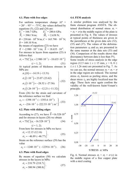
4.1. Plate with free edgesFor uniform temperature change ΔT == 20° – 95° = –75°C, the values defined byequations (5), (22) and (24) are:E * 1 = 166.7 GPa; E * 2 = 280.6 GPa;N = 3961 N/m; M = 2.638 N;TB = 239.66 ⋅ 10 6 N/m; C = 165.790 ⋅ 10 3 N;D = 149.10 N⋅m.By means of equations (23) we havea = -2.980 ⋅ 10 -3 1/m; b = 18.635 ⋅ 10 -6 .For stresses in layers from equation (25) itfollows that:* −3 −6σi = 75Ei ( αi+ 2.980⋅10 z−18.635⋅10)(i = 1, 2). (31)At typical points of thickness stresses inMPa are:σ1( 0)=−14.19 ( −13.51)⎫−3⎪σ1( 1⋅ 10 ) = 23.07 (23.62) ⎪ ⎪⎬. (32)−3σ2 ( 1⋅ 10 ) =−28.52 ( −27.56)⎪−3⎪σ2 ( 1.26⋅ 10 ) =−12.21 ( −11.32)⎪⎭From (26) for the strain and curvature ofthe reference surface we find−6 −6ε0=−1398⋅10 ( −1393.6⋅10 ) ⎫⎪ −3 −3 -1 ⎬ . (33)æ0=−216⋅10 ( −222.53⋅10 ) m ⎪⎭4.2. Plate with sliding edgesAccording to (27), we have b =16.528⋅10 -6and for stresses in layers (28) we obtain* 6σ = 75 ( −16.528⋅10 −iEi αi) (34)(i = 1, 2).From here for stresses in MPa we have:σ1= 12.15 (12.16) ⎫⎬ . (35)σ2=−46.89 ( −46.77)⎭Strain on the reference surface (29) has thevalue−6 −6ε 0=−1240⋅10 ( −1239.6⋅ 10 ) . (36)4.3. Plate with fixed edgesBy means of equation (30) we calculatestresses in the layers in MPa:σ1= 218.79 (218.7) ⎫⎬ . (37)σ2= 300.94 (300.8) ⎭T4.4. FEM analysisA similar problem was analysed by thefinite element program ANSYS. The obtaineddistribution of normal stress σ x == σ y = σ in the middle region of the plate ispresented in Fig. 6. The values of stressesat typical points of thickness are given inthe parentheses at the given data sets (32),(35) and (37). The values of the deformationparameters ε 0 and æ 0 are presented inthe same manner at the data sets (33) and(36). Comparison of the results shows thatdiscrepancy between data is less than 5%.Some results of stress analysis in the edgeregion (12.5 mm ≤ x ≤ 15 mm, y = 0, 0 ≤≤ z ≤ 1.26 mm) are presented in Fig. 7. Aswe can see, the normal stresses σ x = σ y = σin the edge region are reduced. The normalstress σ z , known as peeling stress, and theshear stress τ zx are highly localized near theedge. These facts once again confirm thevalidity of the well-known Saint-Venant’sprinciple.Fig. 6. Normal stresses σ x = σ y = σ (z) inthe middle region of a free copper platewith a steel coating
Page 1 and 2: 6th International DAAAM Baltic Conf
Page 3: a 2 2uz=− ( x + y ) +2z(15)⎡ 2

ANALYSIS OF THERMOELASTIC STRESSES IN LAYERED PLATES

Create successful ePaper yourself

Delete template?

Save as template?