CS229 Lecture Notes - 1

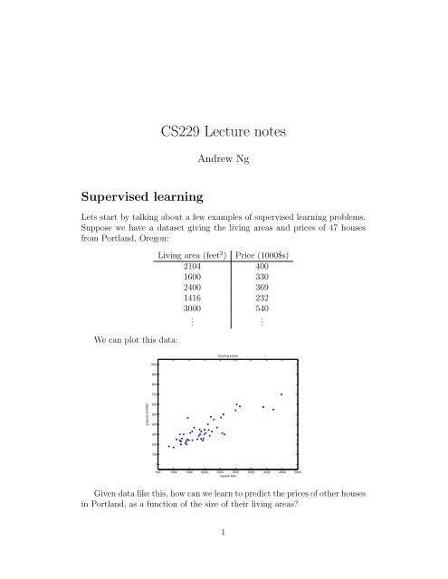
4the training examples we have. To formalize this, we will define a functionthat measures, for each value of the θ’s, how close the h(x (i) )’s are to thecorresponding y (i) ’s. We define the cost function:J(θ) = 1 2m∑(h θ (x (i) ) − y (i) ) 2 .i=1If you’ve seen linear regression before, you may recognize this as the familiarleast-squares cost function that gives rise to the ordinary least squaresregression model. Whether or not you have seen it previously, lets keepgoing, and we’ll eventually show this to be a special case of a much broaderfamily of algorithms.1 LMS algorithmWe want to choose θ so as to minimize J(θ). To do so, lets use a searchalgorithm that starts with some “initial guess” for θ, and that repeatedlychanges θ to make J(θ) smaller, until hopefully we converge to a value ofθ that minimizes J(θ). Specifically, lets consider the gradient descentalgorithm, which starts with some initial θ, and repeatedly performs theupdate:θ j := θ j − α ∂∂θ jJ(θ).(This update is simultaneously performed for all values of j = 0,...,n.)Here, α is called the learning rate. This is a very natural algorithm thatrepeatedly takes a step in the direction of steepest decrease of J.In order to implement this algorithm, we have to work out what is thepartial derivative term on the right hand side. Lets first work it out for thecase of if we have only one training example (x,y), so that we can neglectthe sum in the definition of J. We have:∂∂θ jJ(θ) =∂ 1∂θ j 2 (h θ(x) − y) 2= 2 · 12 (h ∂θ(x) − y) · (h θ (x) − y)∂θ j( n∑)∂= (h θ (x) − y) · θ i x i − y∂θ ji=0= (h θ (x) − y)x j

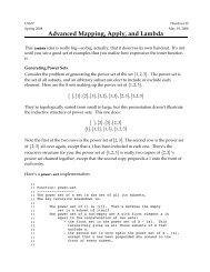
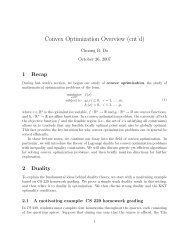
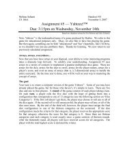
650454035302520151055 10 15 20 25 30 35 40 45 50The ellipses shown above are the contours of a quadratic function. Alsoshown is the trajectory taken by gradient descent, with was initialized at(48,30). The x’s in the figure (joined by straight lines) mark the successivevalues of θ that gradient descent went through.When we run batch gradient descent to fit θ on our previous dataset,to learn to predict housing price as a function of living area, we obtainθ 0 = 71.27, θ 1 = 0.1345. If we plot h θ (x) as a function of x (area), alongwith the training data, we obtain the following figure:housing prices1000900800700price (in $1000)6005004003002001000500 1000 1500 2000 2500 3000 3500 4000 4500 5000square feetIf the number of bedrooms were included as one of the input features as well,we get θ 0 = 89.60,θ 1 = 0.1392, θ 2 = −8.738.The above results were obtained with batch gradient descent. There isan alternative to batch gradient descent that also works very well. Considerthe following algorithm:

82.1 Matrix derivativesFor a function f : R m×n ↦→ R mapping from m-by-n matrices to the realnumbers, we define the derivative of f with respect to A to be:⎡⎤∂f∂f∂A 11· · ·∂A 1n⎢⎥∇ A f(A) = ⎣ .... . ⎦∂f∂A m1· · ·∂f∂A mnThus, the gradient ∇ A f(A) is itself an[ m-by-n matrix, ] whose (i,j)-elementA11 Ais ∂f/∂A ij . For example, suppose A =12is a 2-by-2 matrix, andA 21 A 22the function f : R 2×2 ↦→ R is given byf(A) = 3 2 A 11 + 5A 2 12 + A 21 A 22 .Here, A ij denotes the (i,j) entry of the matrix A. We then have[ ]310A∇ A f(A) =2 12.A 22 A 21We also introduce the trace operator, written “tr.” For an n-by-n(square) matrix A, the trace of A is defined to be the sum of its diagonalentries:n∑trA =If a is a real number (i.e., a 1-by-1 matrix), then tra = a. (If you haven’tseen this “operator notation” before, you should think of the trace of A astr(A), or as application of the “trace” function to the matrix A. It’s morecommonly written without the parentheses, however.)The trace operator has the property that for two matrices A and B suchthat AB is square, we have that trAB = trBA. (Check this yourself!) Ascorollaries of this, we also have, e.g.,i=1A iitrABC = trCAB = trBCA,trABCD = trDABC = trCDAB = trBCDA.The following properties of the trace operator are also easily verified. Here,A and B are square matrices, and a is a real number:trA = trA Ttr(A + B) = trA + trBtraA = atrA

9We now state without proof some facts of matrix derivatives (we won’tneed some of these until later this quarter). Equation (4) applies only tonon-singular square matrices A, where |A| denotes the determinant of A. Wehave:∇ A trAB = B T (1)∇ A Tf(A) = (∇ A f(A)) T (2)∇ A trABA T C = CAB + C T AB T (3)∇ A |A| = |A|(A −1 ) T . (4)To make our matrix notation more concrete, let us now explain in detail themeaning of the first of these equations. Suppose we have some fixed matrixB ∈ R n×m . We can then define a function f : R m×n ↦→ R according tof(A) = trAB. Note that this definition makes sense, because if A ∈ R m×n ,then AB is a square matrix, and we can apply the trace operator to it; thus,f does indeed map from R m×n to R. We can then apply our definition ofmatrix derivatives to find ∇ A f(A), which will itself by an m-by-n matrix.Equation (1) above states that the (i,j) entry of this matrix will be given bythe (i,j)-entry of B T , or equivalently, by B ji .The proofs of Equations (1-3) are reasonably simple, and are left as anexercise to the reader. Equations (4) can be derived using the adjoint representationof the inverse of a matrix. 32.2 Least squares revisitedArmed with the tools of matrix derivatives, let us now proceed to find inclosed-form the value of θ that minimizes J(θ). We begin by re-writing J inmatrix-vectorial notation.Giving a training set, define the design matrix X to be the m-by-nmatrix (actually m-by-n + 1, if we include the intercept term) that contains3 If we define A ′ to be the matrix whose (i,j) element is (−1) i+j times the determinantof the square matrix resulting from deleting row i and column j from A, then it can beproved that A −1 = (A ′ ) T /|A|. (You can check that this is consistent with the standardway of finding A −1 when A is a 2-by-2 matrix. If you want to see a proof of this moregeneral result, see an intermediate or advanced linear algebra text, such as Charles Curtis,1991, Linear Algebra, Springer.) This shows that A ′ = |A|(A −1 ) T . Also, the determinantof a matrix can be written |A| = ∑ j A ijA ′ ij . Since (A′ ) ij does not depend on A ij (as canbe seen from its definition), this implies that (∂/∂A ij )|A| = A ′ ij . Putting all this togethershows the result.

10the training examples’ input values in its rows:⎡⎤— (x (1) ) T —— (x (2) ) T —X = ⎢⎥⎣ . ⎦ .— (x (m) ) T —Also, let ⃗y be the m-dimensional vector containing all the target values fromthe training set:⎡ ⎤y (1)y (2)⃗y = ⎢ ⎥⎣ . ⎦ .y (m)Now, since h θ (x (i) ) = (x (i) ) T θ, we can easily verify that⎡ ⎤ ⎡ ⎤(x (1) ) T θ y (1)⎢ ⎥ ⎢ ⎥Xθ − ⃗y = ⎣ . ⎦ − ⎣ . ⎦(x (m) ) T θ y (m)⎡⎤h θ (x (1) ) − y (1)⎢⎥= ⎣ . ⎦.h θ (x (m) ) − y (m)Thus, using the fact that for a vector z, we have that z T z = ∑ i z2 i :12 (Xθ − ⃗y)T (Xθ − ⃗y) = 1 2m∑(h θ (x (i) ) − y (i) ) 2i=1= J(θ)Finally, to minimize J, lets find its derivatives with respect to θ. CombiningEquations (2) and (3), we find that∇ A T trABA T C = B T A T C T + BA T C (5)

11Hence,1∇ θ J(θ) = ∇ θ2 (Xθ − ⃗y)T (Xθ − ⃗y)= 1 2 ∇ (θ θ T X T Xθ − θ T X T ⃗y − ⃗y T Xθ + ⃗y T ⃗y )= 1 2 ∇ θ tr ( θ T X T Xθ − θ T X T ⃗y − ⃗y T Xθ + ⃗y T ⃗y )= 1 2 ∇ θ(trθ T X T Xθ − 2tr⃗y T Xθ )= 1 (X T Xθ + X T Xθ − 2X T ⃗y )2= X T Xθ − X T ⃗yIn the third step, we used the fact that the trace of a real number is just thereal number; the fourth step used the fact that trA = trA T , and the fifthstep used Equation (5) with A T = θ, B = B T = X T X, and C = I, andEquation (1). To minimize J, we set its derivatives to zero, and obtain thenormal equations:X T Xθ = X T ⃗yThus, the value of θ that minimizes J(θ) is given in closed form by theequationθ = (X T X) −1 X T ⃗y.3 Probabilistic interpretationWhen faced with a regression problem, why might linear regression, andspecifically why might the least-squares cost function J, be a reasonablechoice? In this section, we will give a set of probabilistic assumptions, underwhich least-squares regression is derived as a very natural algorithm.Let us assume that the target variables and the inputs are related via theequationy (i) = θ T x (i) + ǫ (i) ,where ǫ (i) is an error term that captures either unmodeled effects (such asif there are some features very pertinent to predicting housing price, butthat we’d left out of the regression), or random noise. Let us further assumethat the ǫ (i) are distributed IID (independently and identically distributed)according to a Gaussian distribution (also called a Normal distribution) with

12mean zero and some variance σ 2 . We can write this assumption as “ǫ (i) ∼N(0,σ 2 ).” I.e., the density of ǫ (i) is given byp(ǫ (i) ) = √ 1)exp(− (ǫ(i) ) 2.2πσ 2σ 2This implies thatp(y (i) |x (i) ;θ) = √ 1)exp(− (y(i) − θ T x (i) ) 2.2πσ 2σ 2The notation “p(y (i) |x (i) ;θ)” indicates that this is the distribution of y (i)given x (i) and parameterized by θ. Note that we should not condition on θ(“p(y (i) |x (i) ,θ)”), since θ is not a random variable. We can also write thedistribution of y (i) as as y (i) | x (i) ;θ ∼ N(θ T x (i) ,σ 2 ).Given X (the design matrix, which contains all the x (i) ’s) and θ, whatis the distribution of the y (i) ’s? The probability of the data is given byp(⃗y|X;θ). This quantity is typically viewed a function of ⃗y (and perhaps X),for a fixed value of θ. When we wish to explicitly view this as a function ofθ, we will instead call it the likelihood function:L(θ) = L(θ;X,⃗y) = p(⃗y|X;θ).Note that by the independence assumption on the ǫ (i) ’s (and hence also they (i) ’s given the x (i) ’s), this can also be writtenL(θ) ==m∏p(y (i) | x (i) ;θ)i=1m∏i=1)1√ exp(− (y(i) − θ T x (i) ) 2.2πσ 2σ 2Now, given this probabilistic model relating the y (i) ’s and the x (i) ’s, whatis a reasonable way of choosing our best guess of the parameters θ? Theprincipal of maximum likelihood says that we should should choose θ soas to make the data as high probability as possible. I.e., we should choose θto maximize L(θ).Instead of maximizing L(θ), we can also maximize any strictly increasingfunction of L(θ). In particular, the derivations will be a bit simpler if we

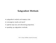
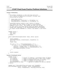
13instead maximize the log likelihood l(θ):l(θ) = log L(θ)m∏)1= log √ exp(− (y(i) − θ T x (i) ) 2i=1 2πσ 2σ 2m∑)1= log √ exp(− (y(i) − θ T x (i) ) 22πσ 2σ 2i=1= m log1√2πσ− 1 σ 2 · 12m∑(y (i) − θ T x (i) ) 2 .Hence, maximizing l(θ) gives the same answer as minimizing12i=1m∑(y (i) − θ T x (i) ) 2 ,i=1which we recognize to be J(θ), our original least-squares cost function.To summarize: Under the previous probabilistic assumptions on the data,least-squares regression corresponds to finding the maximum likelihood estimateof θ. This is thus one set of assumptions under which least-squares regressioncan be justified as a very natural method that’s just doing maximumlikelihood estimation. (Note however that the probabilistic assumptions areby no means necessary for least-squares to be a perfectly good and rationalprocedure, and there may—and indeed there are—other natural assumptionsthat can also be used to justify it.)Note also that, in our previous discussion, our final choice of θ did notdepend on what was σ 2 , and indeed we’d have arrived at the same resulteven if σ 2 were unknown. We will use this fact again later, when we talkabout the exponential family and generalized linear models.4 Locally weighted linear regressionConsider the problem of predicting y from x ∈ R. The leftmost figure belowshows the result of fitting a y = θ 0 + θ 1 x to a dataset. We see that the datadoesn’t really lie on straight line, and so the fit is not very good.

yyy144.54.54.54443.53.53.53332.52.52.52221.51.51.51110.50.50.500 1 2 3 4 5 6 7x00 1 2 3 4 5 6 7x00 1 2 3 4 5 6 7xInstead, if we had added an extra feature x 2 , and fit y = θ 0 + θ 1 x + θ 2 x 2 ,then we obtain a slightly better fit to the data. (See middle figure) Naively, itmight seem that the more features we add, the better. However, there is alsoa danger in adding too many features: The rightmost figure is the result offitting a 5-th order polynomial y = ∑ 5j=0 θ jx j . We see that even though thefitted curve passes through the data perfectly, we would not expect this tobe a very good predictor of, say, housing prices (y) for different living areas(x). Without formally defining what these terms mean, we’ll say the figureon the left shows an instance of underfitting—in which the data clearlyshows structure not captured by the model—and the figure on the right isan example of overfitting. (Later in this class, when we talk about learningtheory we’ll formalize some of these notions, and also define more carefullyjust what it means for a hypothesis to be good or bad.)As discussed previously, and as shown in the example above, the choice offeatures is important to ensuring good performance of a learning algorithm.(When we talk about model selection, we’ll also see algorithms for automaticallychoosing a good set of features.) In this section, let us talk briefly talkabout the locally weighted linear regression (LWR) algorithm which, assumingthere is sufficient training data, makes the choice of features less critical.This treatment will be brief, since you’ll get a chance to explore some of theproperties of the LWR algorithm yourself in the homework.In the original linear regression algorithm, to make a prediction at a querypoint x (i.e., to evaluate h(x)), we would:1. Fit θ to minimize ∑ i (y(i) − θ T x (i) ) 2 .2. Output θ T x.In contrast, the locally weighted linear regression algorithm does the following:1. Fit θ to minimize ∑ i w(i) (y (i) − θ T x (i) ) 2 .2. Output θ T x.

15Here, the w (i) ’s are non-negative valued weights. Intuitively, if w (i) is largefor a particular value of i, then in picking θ, we’ll try hard to make (y (i) −θ T x (i) ) 2 small. If w (i) is small, then the (y (i) − θ T x (i) ) 2 error term will bepretty much ignored in the fit.A fairly standard choice for the weights is 4)w (i) = exp(− (x(i) − x) 22τ 2Note that the weights depend on the particular point x at which we’re tryingto evaluate x. Moreover, if |x (i) − x| is small, then w (i) is close to 1; andif |x (i) − x| is large, then w (i) is small. Hence, θ is chosen giving a muchhigher “weight” to the (errors on) training examples close to the query pointx. (Note also that while the formula for the weights takes a form that iscosmetically similar to the density of a Gaussian distribution, the w (i) ’s donot directly have anything to do with Gaussians, and in particular the w (i)are not random variables, normally distributed or otherwise.) The parameterτ controls how quickly the weight of a training example falls off with distanceof its x (i) from the query point x; τ is called the bandwidth parameter, andis also something that you’ll get to experiment with in your homework.Locally weighted linear regression is the first example we’re seeing of anon-parametric algorithm. The (unweighted) linear regression algorithmthat we saw earlier is known as a parametric learning algorithm, becauseit has a fixed, finite number of parameters (the θ i ’s), which are fit to thedata. Once we’ve fit the θ i ’s and stored them away, we no longer need tokeep the training data around to make future predictions. In contrast, tomake predictions using locally weighted linear regression, we need to keepthe entire training set around. The term “non-parametric” (roughly) refersto the fact that the amount of stuff we need to keep in order to represent thehypothesis h grows linearly with the size of the training set.4 If x is vector-valued, this is generalized to be w (i) = exp(−(x (i) −x) T (x (i) −x)/(2τ 2 )),or w (i) = exp(−(x (i) − x) T Σ −1 (x (i) − x)/2), for an appropriate choice of τ or Σ.

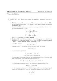
16Part IIClassification and logisticregressionLets now talk about the classification problem. This is just like the regressionproblem, except that the values y we now want to predict take on onlya small number of discrete values. For now, we will focus on the binaryclassification problem in which y can take on only two values, 0 and 1.(Most of what we say here will also generalize to the multiple-class case.)For instance, if we are trying to build a spam classifier for email, then x (i)may be some features of a piece of email, and y may be 1 if it is a pieceof spam mail, and 0 otherwise. 0 is also called the negative class, and 1the positive class, and they are sometimes also denoted by the symbols “-”and “+.” Given x (i) , the corresponding y (i) is also called the label for thetraining example.5 Logistic regressionWe could approach the classification problem ignoring the fact that y isdiscrete-valued, and use our old linear regression algorithm to try to predicty given x. However, it is easy to construct examples where this methodperforms very poorly. Intuitively, it also doesn’t make sense for h θ (x) to takevalues larger than 1 or smaller than 0 when we know that y ∈ {0, 1}.To fix this, lets change the form for our hypotheses h θ (x). We will chooseh θ (x) = g(θ T x) =11 + e −θT x ,where1g(z) =1 + e −zis called the logistic function or the sigmoid function. Here is a plotshowing g(z):

1710.90.80.70.6g(z)0.50.40.30.20.10−5 −4 −3 −2 −1 0 1 2 3 4 5zNotice that g(z) tends towards 1 as z → ∞, and g(z) tends towards 0 asz → −∞. Moreover, g(z), and hence also h(x), is always bounded between0 and 1. As before, we are keeping the convention of letting x 0 = 1, so thatθ T x = θ 0 + ∑ nj=1 θ jx j .For now, lets take the choice of g as given. Other functions that smoothlyincrease from 0 to 1 can also be used, but for a couple of reasons that we’ll seelater (when we talk about GLMs, and when we talk about generative learningalgorithms), the choice of the logistic function is a fairly natural one. Beforemoving on, here’s a useful property of the derivative of the sigmoid function,which we write a g ′ :g ′ (z) =d 1dz 1 + e −z1 (=)e−z(1 + e −z ) 2 ( )1=(1 + e −z ) · 11 −(1 + e −z )= g(z)(1 − g(z)).So, given the logistic regression model, how do we fit θ for it? Followinghow we saw least squares regression could be derived as the maximumlikelihood estimator under a set of assumptions, lets endow our classificationmodel with a set of probabilistic assumptions, and then fit the parametersvia maximum likelihood.

18Let us assume thatP(y = 1 | x;θ) = h θ (x)P(y = 0 | x;θ) = 1 − h θ (x)Note that this can be written more compactly asp(y | x;θ) = (h θ (x)) y (1 − h θ (x)) 1−yAssuming that the m training examples were generated independently, wecan then write down the likelihood of the parameters asL(θ) = p(⃗y | X;θ)m∏= p(y (i) | x (i) ;θ)=i=1m∏ (hθ (x (i) ) ) y (i) ( 1 − h θ (x (i) ) ) 1−y (i)i=1As before, it will be easier to maximize the log likelihood:l(θ) = log L(θ)m∑= y (i) log h(x (i) ) + (1 − y (i) ) log(1 − h(x (i) ))i=1How do we maximize the likelihood? Similar to our derivation in the caseof linear regression, we can use gradient ascent. Written in vectorial notation,our updates will therefore be given by θ := θ + α∇ θ l(θ). (Note the positiverather than negative sign in the update formula, since we’re maximizing,rather than minimizing, a function now.) Lets start by working with justone training example (x,y), and take derivatives to derive the stochasticgradient ascent rule:∂∂θ jl(θ) ==()1yg(θ T x) − (1 − y) 1 ∂g(θ T x)1 − g(θ T x) ∂θ j()1yg(θ T x) − (1 − y) 1g(θ T x)(1 − g(θ T x) ∂ θ T x1 − g(θ T x)∂θ j= ( y(1 − g(θ T x)) − (1 − y)g(θ T x) ) x j= (y − h θ (x))x j

19Above, we used the fact that g ′ (z) = g(z)(1 − g(z)). This therefore gives usthe stochastic gradient ascent ruleθ j := θ j + α ( y (i) − h θ (x (i) ) ) x (i)jIf we compare this to the LMS update rule, we see that it looks identical; butthis is not the same algorithm, because h θ (x (i) ) is now defined as a non-linearfunction of θ T x (i) . Nonetheless, it’s a little surprising that we end up withthe same update rule for a rather different algorithm and learning problem.Is this coincidence, or is there a deeper reason behind this? We’ll answer thiswhen get get to GLM models. (See also the extra credit problem on Q3 ofproblem set 1.)6 Digression: The perceptron learning algorithmWe now digress to talk briefly about an algorithm that’s of some historicalinterest, and that we will also return to later when we talk about learningtheory. Consider modifying the logistic regression method to “force” it tooutput values that are either 0 or 1 or exactly. To do so, it seems natural tochange the definition of g to be the threshold function:{ 1 if z ≥ 0g(z) =0 if z < 0If we then let h θ (x) = g(θ T x) as before but using this modified definition ofg, and if we use the update ruleθ j := θ j + α ( y (i) − h θ (x (i) ) ) x (i)j .then we have the perceptron learning algorithm.In the 1960s, this “perceptron” was argued to be a rough model for howindividual neurons in the brain work. Given how simple the algorithm is, itwill also provide a starting point for our analysis when we talk about learningtheory later in this class. Note however that even though the perceptron maybe cosmetically similar to the other algorithms we talked about, it is actuallya very different type of algorithm than logistic regression and least squareslinear regression; in particular, it is difficult to endow the perceptron’s predictionswith meaningful probabilistic interpretations, or derive the perceptronas a maximum likelihood estimation algorithm.

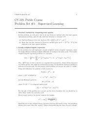
207 Another algorithm for maximizing l(θ)Returning to logistic regression with g(z) being the sigmoid function, letsnow talk about a different algorithm for minimizing l(θ).To get us started, lets consider Newton’s method for finding a zero of afunction. Specifically, suppose we have some function f : R ↦→ R, and wewish to find a value of θ so that f(θ) = 0. Here, θ ∈ R is a real number.Newton’s method performs the following update:θ := θ − f(θ)f ′ (θ) .This method has a natural interpretation in which we can think of it asapproximating the function f via a linear function that is tangent to f atthe current guess θ, solving for where that linear function equals to zero, andletting the next guess for θ be where that linear function is zero.Here’s a picture of the Newton’s method in action:606060505050404040303030f(x)f(x)f(x)202020101010000−101 1.5 2 2.5 3 3.5 4 4.5 5x−101 1.5 2 2.5 3 3.5 4 4.5 5x−101 1.5 2 2.5 3 3.5 4 4.5 5xIn the leftmost figure, we see the function f plotted along with the liney = 0. We’re trying to find θ so that f(θ) = 0; the value of θ that achieves thisis about 1.3. Suppose we initialized the algorithm with θ = 4.5. Newton’smethod then fits a straight line tangent to f at θ = 4.5, and solves for thewhere that line evaluates to 0. (Middle figure.) This give us the next guessfor θ, which is about 2.8. The rightmost figure shows the result of runningone more iteration, which the updates θ to about 1.8. After a few moreiterations, we rapidly approach θ = 1.3.Newton’s method gives a way of getting to f(θ) = 0. What if we want touse it to maximize some function l? The maxima of l correspond to pointswhere its first derivative l ′ (θ) is zero. So, by letting f(θ) = l ′ (θ), we can usethe same algorithm to maximize l, and we obtain update rule:θ := θ − l′ (θ)l ′′ (θ) .(Something to think about: How would this change if we wanted to useNewton’s method to minimize rather than maximize a function?)

21Lastly, in our logistic regression setting, θ is vector-valued, so we need togeneralize Newton’s method to this setting. The generalization of Newton’smethod to this multidimensional setting (also called the Newton-Raphsonmethod) is given byθ := θ − H −1 ∇ θ l(θ).Here, ∇ θ l(θ) is, as usual, the vector of partial derivatives of l(θ) with respectto the θ i ’s; and H is an n-by-n matrix (actually, n + 1-by-n + 1, assumingthat we include the intercept term) called the Hessian, whose entries aregiven byH ij = ∂2 l(θ)∂θ i ∂θ j.Newton’s method typically enjoys faster convergence than (batch) gradientdescent, and requires many fewer iterations to get very close to theminimum. One iteration of Newton’s can, however, be more expensive thanone iteration of gradient descent, since it requires finding and inverting ann-by-n Hessian; but so long as n is not too large, it is usually much fasteroverall. When Newton’s method is applied to maximize the logistic regressionlog likelihood function l(θ), the resulting method is also called Fisherscoring.

22Part IIIGeneralized Linear Models 5So far, we’ve seen a regression example, and a classification example. In theregression example, we had y|x;θ ∼ N(µ,σ 2 ), and in the classification one,y|x;θ ∼ Bernoulli(φ), where for some appropriate definitions of µ and φ asfunctions of x and θ. In this section, we will show that both of these methodsare special cases of a broader family of models, called Generalized LinearModels (GLMs). We will also show how other models in the GLM familycan be derived and applied to other classification and regression problems.8 The exponential familyTo work our way up to GLMs, we will begin by defining exponential familydistributions. We say that a class of distributions is in the exponential familyif it can be written in the formp(y;η) = b(y) exp(η T T(y) − a(η)) (6)Here, η is called the natural parameter (also called the canonical parameter)of the distribution; T(y) is the sufficient statistic (for the distributionswe consider, it will often be the case that T(y) = y); and a(η) is the logpartition function. The quantity e −a(η) essentially plays the role of a normalizationconstant, that makes sure the distribution p(y;η) sums/integratesover y to 1.A fixed choice of T, a and b defines a family (or set) of distributions thatis parameterized by η; as we vary η, we then get different distributions withinthis family.We now show that the Bernoulli and the Gaussian distributions are examplesof exponential family distributions. The Bernoulli distribution withmean φ, written Bernoulli(φ), specifies a distribution over y ∈ {0, 1}, so thatp(y = 1;φ) = φ; p(y = 0;φ) = 1 − φ. As we varying φ, we obtain Bernoullidistributions with different means. We now show that this class of Bernoullidistributions, ones obtained by varying φ, is in the exponential family; i.e.,that there is a choice of T, a and b so that Equation (6) becomes exactly theclass of Bernoulli distributions.5 The presentation of the material in this section takes inspiration from Michael I.Jordan, Learning in graphical models (unpublished book draft), and also McCullagh andNelder, Generalized Linear Models (2nd ed.).

23We write the Bernoulli distribution as:p(y;φ) = φ y (1 − φ) 1−y= exp(y log φ + (1 − y) log(1 − φ))(( ( )) )φ= exp log y + log(1 − φ) .1 − φThus, the natural parameter is given by η = log(φ/(1 − φ)). Interestingly, ifwe invert this definition for η by solving for φ in terms of η, we obtain φ =1/(1 + e −η ). This is the familiar sigmoid function! This will come up againwhen we derive logistic regression as a GLM. To complete the formulationof the Bernoulli distribution as an exponential family distribution, we alsohaveT(y) = ya(η) = − log(1 − φ)b(y) = 1= log(1 + e η )This shows that the Bernoulli distribution can be written in the form ofEquation (6), using an appropriate choice of T, a and b.Lets now move on to consider the Gaussian distribution. Recall that,when deriving linear regression, the value of σ 2 had no effect on our finalchoice of θ and h θ (x). Thus, we can choose an arbitrary value for σ 2 withoutchanging anything. To simplify the derivation below, lets set σ 2 = 1. 6 Wethen have:1p(y;µ) = √ exp(− 1 )2π 2 (y − µ)2=1√ exp(− 1 )2π 2 y2· exp(µy − 1 )2 µ26 If we leave σ 2 as a variable, the Gaussian distribution can also be shown to be in theexponential family, where η ∈ R 2 is now a 2-dimension vector that depends on both µ andσ. For the purposes of GLMs, however, the σ 2 parameter can also be treated by consideringa more general definition of the exponential family: p(y;η,τ) = b(a,τ)exp((η T T(y) −a(η))/c(τ)). Here, τ is called the dispersion parameter, and for the Gaussian, c(τ) = σ 2 ;but given our simplification above, we won’t need the more general definition for theexamples we will consider here.

24Thus, we see that the Gaussian is in the exponential family, withη = µT(y) = ya(η) = µ 2 /2= η 2 /2b(y) = (1/ √ 2π) exp(−y 2 /2).There’re many other distributions that are members of the exponentialfamily: The multinomial (which we’ll see later), the Poisson (for modellingcount-data; also see the problem set); the gamma and the exponential(for modelling continuous, non-negative random variables, such as timeintervals);the beta and the Dirichlet (for distributions over probabilities);and many more. In the next section, we will describe a general “recipe”for constructing models in which y (given x and θ) comes from any of thesedistributions.9 Constructing GLMsSuppose you would like to build a model to estimate the number y of customersarriving in your store (or number of page-views on your website) inany given hour, based on certain features x such as store promotions, recentadvertising, weather, day-of-week, etc. We know that the Poisson distributionusually gives a good model for numbers of visitors. Knowing this, howcan we come up with a model for our problem? Fortunately, the Poisson is anexponential family distribution, so we can apply a Generalized Linear Model(GLM). In this section, we will we will describe a method for constructingGLM models for problems such as these.More generally, consider a classification or regression problem where wewould like to predict the value of some random variable y as a function ofx. To derive a GLM for this problem, we will make the following threeassumptions about the conditional distribution of y given x and about ourmodel:1. y | x;θ ∼ ExponentialFamily(η). I.e., given x and θ, the distribution ofy follows some exponential family distribution, with parameter η.2. Given x, our goal is to predict the expected value of T(y) given x.In most of our examples, we will have T(y) = y, so this means wewould like the prediction h(x) output by our learned hypothesis h to

25satisfy h(x) = E[y|x]. (Note that this assumption is satisfied in thechoices for h θ (x) for both logistic regression and linear regression. Forinstance, in logistic regression, we had h θ (x) = p(y = 1|x;θ) = 0 · p(y =0|x;θ) + 1 · p(y = 1|x;θ) = E[y|x;θ].)3. The natural parameter η and the inputs x are related linearly: η = θ T x.(Or, if η is vector-valued, then η i = θ T i x.)The third of these assumptions might seem the least well justified ofthe above, and it might be better thought of as a “design choice” in ourrecipe for designing GLMs, rather than as an assumption per se. Thesethree assumptions/design choices will allow us to derive a very elegant classof learning algorithms, namely GLMs, that have many desirable propertiessuch as ease of learning. Furthermore, the resulting models are often veryeffective for modelling different types of distributions over y; for example, wewill shortly show that both logistic regression and ordinary least squares canboth be derived as GLMs.9.1 Ordinary Least SquaresTo show that ordinary least squares is a special case of the GLM familyof models, consider the setting where the target variable y (also called theresponse variable in GLM terminology) is continuous, and we model theconditional distribution of y given x as as a Gaussian N(µ,σ 2 ). (Here, µmay depend x.) So, we let the ExponentialFamily(η) distribution above bethe Gaussian distribution. As we saw previously, in the formulation of theGaussian as an exponential family distribution, we had µ = η. So, we haveh θ (x) = E[y|x;θ]= µ= η= θ T x.The first equality follows from Assumption 2, above; the second equalityfollows from the fact that y|x;θ ∼ N(µ,σ 2 ), and so its expected value is givenby µ; the third equality follows from Assumption 1 (and our earlier derivationshowing that µ = η in the formulation of the Gaussian as an exponentialfamily distribution); and the last equality follows from Assumption 3.

269.2 Logistic RegressionWe now consider logistic regression. Here we are interested in binary classification,so y ∈ {0, 1}. Given that y is binary-valued, it therefore seems naturalto choose the Bernoulli family of distributions to model the conditional distributionof y given x. In our formulation of the Bernoulli distribution asan exponential family distribution, we had φ = 1/(1 + e −η ). Furthermore,note that if y|x;θ ∼ Bernoulli(φ), then E[y|x;θ] = φ. So, following a similarderivation as the one for ordinary least squares, we get:h θ (x) = E[y|x;θ]= φ= 1/(1 + e −η )= 1/(1 + e −θT x )So, this gives us hypothesis functions of the form h θ (x) = 1/(1 + e −θT x ). Ifyou are previously wondering how we came up with the form of the logisticfunction 1/(1 + e −z ), this gives one answer: Once we assume that y conditionedon x is Bernoulli, it arises as a consequence of the definition of GLMsand exponential family distributions.To introduce a little more terminology, the function g giving the distribution’smean as a function of the natural parameter (g(η) = E[T(y);η])is called the canonical response function. Its inverse, g −1 , is called thecanonical link function. Thus, the canonical response function for theGaussian family is just the identify function; and the canonical responsefunction for the Bernoulli is the logistic function. 79.3 Softmax RegressionLets look at one more example of a GLM. Consider a classification problemin which the response variable y can take on any one of k values, so y ∈{1 2,...,k}. For example, rather than classifying email into the two classesspam or not-spam—which would have been a binary classification problem—we might want to classify it into three classes, such as spam, personal mail,and work-related mail. The response variable is still discrete, but can nowtake on more than two values. We will thus model it as distributed accordingto a multinomial distribution.7 Many texts use g to denote the link function, and g −1 to denote the response function;but the notation we’re using here, inherited from the early machine learning literature,will be more consistent with the notation used in the rest of the class.

27Lets derive a GLM for modelling this type of multinomial data. To doso, we will begin by expressing the multinomial as an exponential familydistribution.To parameterize a multinomial over k possible outcomes, one could usek parameters φ 1 ,...,φ k specifying the probability of each of the outcomes.However, these parameters would be redundant, or more formally, they wouldnot be independent (since knowing any k −1 of the φ i ’s uniquely determinesthe last one, as they must satisfy ∑ ki=1 φ i = 1). So, we will instead parameterizethe multinomial with only k − 1 parameters, φ 1 ,...,φ k−1 , whereφ i = p(y = i;φ), and p(y = k;φ) = 1 − ∑ k−1i=1 φ i. For notational convenience,we will also let φ k = 1 − ∑ k−1i=1 φ i, but we should keep in mind that this isnot a parameter, and that it is fully specified by φ 1 ,...,φ k−1 .To express the multinomial as an exponential family distribution, we willdefine T(y) ∈ R k−1 as follows:⎡T(1) =⎢⎣100.0⎤⎡, T(2) =⎥ ⎢⎦ ⎣010.0⎤⎡, T(3) =⎥ ⎢⎦ ⎣001.0⎤⎡, · · · ,T(k−1) =⎥⎢⎦⎣000.1⎤⎡, T(k) =⎥ ⎢⎦ ⎣Unlike our previous examples, here we do not have T(y) = y; also, T(y) isnow a k − 1 dimensional vector, rather than a real number. We will write(T(y)) i to denote the i-th element of the vector T(y).We introduce one more very useful piece of notation. An indicator function1{·} takes on a value of 1 if its argument is true, and 0 otherwise(1{True} = 1, 1{False} = 0). For example, 1{2 = 3} = 0, and 1{3 =5 − 2} = 1. So, we can also write the relationship between T(y) and y as(T(y)) i = 1{y = i}. (Before you continue reading, please make sure you understandwhy this is true!) Further, we have that E[(T(y)) i ] = P(y = i) = φ i .We are now ready to show that the multinomial is a member of the000.0⎤,⎥⎦

28exponential family. We have:wherep(y;φ) = φ 1{y=1}1 φ 1{y=2}2 · · ·φ 1{y=k}k= φ 1{y=1}1 φ 1{y=2}2 · · ·φ 1−P k−1ki=1 1{y=i}= φ (T(y)) 11 φ (T(y)) 22 · · ·φ 1−P k−1i=1 (T(y)) ik= exp((T(y)) 1 log(φ 1 ) + (T(y)) 2 log(φ 2 ) +(· · · + 1 − ∑ )k−1i=1 (T(y)) i log(φ k ))= exp((T(y)) 1 log(φ 1 /φ k ) + (T(y)) 2 log(φ 2 /φ k ) +· · · + (T(y)) k−1 log(φ k−1 /φ k ) + log(φ k ))= b(y) exp(η T T(y) − a(η))η =⎡⎢⎣log(φ 1 /φ k )log(φ 2 /φ k ).log(φ k−1 /φ k )a(η) = − log(φ k )b(y) = 1.This completes our formulation of the multinomial as an exponential familydistribution.The link function is given (for i = 1,...,k) byη i = log φ iφ k.For convenience, we have also defined η k = log(φ k /φ k ) = 0. To invert thelink function and derive the response function, we therefore have thatφ k⎤⎥⎦ ,e η i= φ iφ kφ k e η i= φ i (7)k∑ k∑e η i= φ i = 1i=1This implies that φ k = 1/ ∑ ki=1 eη i, which can be substituted back into Equation(7) to give the response functionφ i =i=1e η i∑ kj=1 eη j

29This function mapping from the η’s to the φ’s is called the softmax function.To complete our model, we use Assumption 3, given earlier, that the η i ’sare linearly related to the x’s. So, have η i = θi T x (for i = 1,...,k − 1),where θ 1 ,...,θ k−1 ∈ R n+1 are the parameters of our model. For notationalconvenience, we can also define θ k = 0, so that η k = θk T x = 0, as givenpreviously. Hence, our model assumes that the conditional distribution of ygiven x is given byp(y = i|x;θ) = φ ie η i= ∑ kj=1 eη j=e θT i x∑ kj=1 eθT j x (8)This model, which applies to classification problems where y ∈ {1,...,k}, iscalled softmax regression. It is a generalization of logistic regression.Our hypothesis will outputh θ (x) = E[T(y)|x;θ]⎡⎤1{y = 1}1{y = 2}= E⎢x;θ⎥⎣ .⎦1{y = k − 1} ∣⎡ ⎤φ 1φ 2= ⎢ ⎥⎣ . ⎦φ k−1⎡=⎢⎣⎤exp(θ1 T P x)kj=1 exp(θT j x)exp(θ2 T P x)k j=1 exp(θT j x). ⎥⎦exp(θk−1 T P x)kj=1 exp(θT j x)In other words, our hypothesis will output the estimated probability thatp(y = i|x;θ), for every value of i = 1,...,k. (Even though h θ (x) as definedabove is only k − 1 dimensional, clearly p(y = k|x;θ) can be obtained as1 − ∑ k−1i=1 φ i.).

30Lastly, lets discuss parameter fitting. Similar to our original derivation ofordinary least squares and logistic regression, if we have a training set of mexamples {(x (i) ,y (i) );i = 1,...,m} and would like to learn the parameters θ iof this model, we would begin by writing down the log-likelihoodl(θ) ==m∑log p(y (i) |x (i) ;θ)i=1m∑logi=1( ) 1{y k∏(i) =l}e θT l x(i)∑ kj=1 eθT j x(i)l=1To obtain the second line above, we used the definition for p(y|x;θ) givenin Equation (8). We can now obtain the maximum likelihood estimate ofthe parameters by maximizing l(θ) in terms of θ, using a method such asgradient ascent or Newton’s method.