cvx Users' Guide - Stanford Engineering Everywhere - Stanford ...

cvx Users’ Guidefor cvx version 1.2 (build 667)Michael Grantmcgrant@stanford.eduYinyu Yeyyye@stanford.eduJune 24, 2008Stephen Boydboyd@stanford.edu1

8 Advanced topics 448.1 Solver selection . . . . . . . . . . . . . . . . . . . . . . . . . . . . . . 448.2 Controlling solver precision . . . . . . . . . . . . . . . . . . . . . . . . 448.3 Miscellaneous cvx commands . . . . . . . . . . . . . . . . . . . . . . 468.4 Assignments versus equality constraints . . . . . . . . . . . . . . . . . 468.5 Indexed dual variables . . . . . . . . . . . . . . . . . . . . . . . . . . 48A Installation and compatability 50A.1 Basic instructions . . . . . . . . . . . . . . . . . . . . . . . . . . . . . 50A.2 MEX file compilation . . . . . . . . . . . . . . . . . . . . . . . . . . . 51A.3 About SeDuMi and SDPT3 . . . . . . . . . . . . . . . . . . . . . . . 51A.4 A Matlab 7.0 issue . . . . . . . . . . . . . . . . . . . . . . . . . . . . 52B Operators, functions, and sets 53B.1 Basic operators and linear functions . . . . . . . . . . . . . . . . . . . 53B.2 Nonlinear functions . . . . . . . . . . . . . . . . . . . . . . . . . . . . 54B.3 Sets . . . . . . . . . . . . . . . . . . . . . . . . . . . . . . . . . . . . 59C cvx status messages 61D Advanced solver topics 63D.1 The successive approximation method . . . . . . . . . . . . . . . . . . 63D.2 Irrational powers . . . . . . . . . . . . . . . . . . . . . . . . . . . . . 63D.3 Overdetermined problems . . . . . . . . . . . . . . . . . . . . . . . . 64E Acknowledgements 653

1 Introduction1.1 What is cvx?cvx is a modeling system for disciplined convex programming. Disciplined convex programs,or DCPs, are convex optimization problems that are described using a limitedset of construction rules, which enables them to be analyzed and solved efficiently.cvx can solve standard problems such as linear programs (LPs), quadratic programs(QPs), second-order cone programs (SOCPs), and semidefinite programs (SDPs);but compared to directly using a solver for one or these types of problems, cvx cangreatly simplify the task of specifying the problem. cvx can also solve much morecomplex convex optimization problems, including many involving nondifferentiablefunctions, such as l 1 norms. You can use cvx to conveniently formulate and solveconstrained norm minimization, entropy maximization, determinant maximization,and many other problems.To use cvx effectively, you need to know at least a bit about convex optimization.For background on convex optimization, see the book Convex Optimization[BV04], available on-line at www.stanford.edu/~boyd/cvxbook/, or the Stanfordcourse EE364A, available at www.stanford.edu/class/ee364a/.cvx is implemented in Matlab [Mat04], effectively turning Matlab into an optimizationmodeling language. Model specifications are constructed using commonMatlab operations and functions, and standard Matlab code can be freely mixed withthese specifications. This combination makes it simple to perform the calculationsneeded to form optimization problems, or to process the results obtained from theirsolution. For example, it is easy to compute an optimal trade-off curve by formingand solving a family of optimization problems by varying the constraints. As anotherexample, cvx can be used as a component of a larger system that uses convex optimization,such as a branch and bound method, or an engineering design framework.cvx also provides special modes to simplify the construction of problems from twospecific problem classes. In SDP mode, cvx applies a matrix interpretation to theinequality operator, so that linear matrix inequalities (LMIs) and SDPs may be expressedin a more natural form. In GP mode, cvx accepts all of the special functionsand combination rules of geometric programming, including monomials, posynomials,and generalized posynomials, and transforms such problems into convex formso that they can be solved efficiently. For background on geometric programming,see the tutorial paper [BKVH05], available at www.stanford.edu/~boyd/papers/gp_tutorial.html.cvx was designed and implemented by Michael Grant, with input from StephenBoyd and Yinyu Ye [GBY06]. It incorporates ideas from earlier work by Löfberg[Löf05], Dahl and Vandenberghe [DV05], Crusius [Cru02], Wu and Boyd [WB00], andmany others. The modeling language follows the spirit of AMPL [FGK99] or GAMS[BKMR98]; unlike these packages, however, cvx was designed from the beginning tofully exploit convexity. The specific method for implementing cvx in Matlab drawsheavily from YALMIP [Löf05]. We also hope to develop versions of cvx for otherplatforms in the future.4

1.2 What is disciplined convex programming?Disciplined convex programming is a methodology for constructing convex optimizationproblems proposed by Michael Grant, Stephen Boyd, and Yinyu Ye [GBY06,Gra04]. It is meant to support the formulation and construction of optimizationproblems that the user intends from the outset to be convex. Disciplined convexprogramming imposes a set of conventions or rules, which we call the DCP ruleset.Problems which adhere to the ruleset can be rapidly and automatically verified asconvex and converted to solvable form. Problems that violate the ruleset are rejected,even when the problem is convex. That is not to say that such problems cannot besolved using DCP; they just need to be rewritten in a way that conforms to the DCPruleset.A detailed description of the DCP ruleset is given in §4, and it is important foranyone who intends to actively use cvx to understand it. The ruleset is simple tolearn, and is drawn from basic principles of convex analysis. In return for acceptingthe restrictions imposed by the ruleset, we obtain considerable benefits, such asautomatic conversion of problems to solvable form, and full support for nondifferentiablefunctions. In practice, we have found that disciplined convex programs closelyresemble their natural mathematical forms.1.3 About this versionSupported solvers. This version of cvx supports two core solvers, SeDuMi [Stu99]and SDPT3 [TTT06], which is the default. Future versions of cvx may support othersolvers, such as MOSEK [MOS05] or CVXOPT [DV05]. SeDuMi and SDPT3 areopen-source interior-point solvers written in Matlab for LPs, SOCPs, SDPs, andcombinations thereof.Problems handled exactly. cvx will convert the specified problem to an LP,SOCP, or SDP, when all the functions in the problem specification can be representedin these forms. This includes a wide variety of functions, such as minimum andmaximum, absolute value, quadratic forms, the minimum and maximum eigenvaluesof a symmetric matrix, power functions x p , and l p norms (both for p rational).Problems handled with (good) approximations. For a few functions, cvx willmake a (good) approximation to transform the specified problem to one that canbe handled by a combined LP, SOCP, and SDP solver. For example, when a powerfunction or l p -norm is used, with non-rational exponent p, cvx replaces p with anearby rational. The log of the normal cumulative distribution log Φ(x) is replacedwith an SDP-compatible approximation.Problems handled with successive approximation. This version of cvx addssupport for a number of functions that cannot be exactly represented via LP, SOCP, orSDP, including log, exp, log-sum-exp log(expx 1 +· · ·+exp x n ), entropy, and Kullback-Leibler divergence. These problems are handled by solving a sequence (typically just5

a handful) of SDPs, which yields the solution to the full accuracy of the core solver.On the other hand, this technique can be substantially slower than if the core solverdirectly handled such functions. The successive approximation method is brieflydescribed in Appendix D.1. Geometric problems are now solved in this manner aswell; in previous versions, an approximation was made.Ultimately, we will interfacecvx to a solver with native support for such functions,which result in a large speedup in solving problems with these functions. Until then,users should be aware that problems involving these functions can be slow to solveusing the current version of cvx. For this reason, when one of these functions is used,the user will be warned that the successive approximate technique will be used.We emphasize that most users do not need to know howcvx handles their problem;what matters is what functions and operations can be handled. For a full list offunctions supported by cvx, see Appendix B, or use the online help function bytyping help cvx/builtins (for functions already in Matlab, such as sqrt or log) orhelp cvx/functions (for functions not in Matlab, such as lambda_max).1.4 FeedbackPlease contact Michael Grant (mcgrant@stanford.edu) or Stephen Boyd (boyd@stanford.edu)with your comments. If you discover what you think is a bug, please include the followingin your communication, so we can reproduce and fix the problem:• the cvx model and supporting data that caused the error• a copy of any error messages that it produced• the cvx version number and build number• the version number of Matlab that you are running• the name and version of the operating system you are usingThe latter three items can all be discovered by typingcvx_versionat the MATLAB command prompt; simply copy its output into your email message.1.5 What cvx is notcvx is not meant to be a tool for checking if your problem is convex. You need toknow a bit about convex optimization to effectively use cvx; otherwise you are theproverbial monkey at the typewriter, hoping to (accidently) type in a valid disciplinedconvex program.On the other hand, if cvx accepts your problem, you can be sure it is convex. Inconjunction with a course on (or self study of) convex optimization, cvx (especially,its error messages) can be very helpful in learning some basic convex analysis. While6

cvx will attempt to give helpful error messages when you violate the DCP ruleset, itcan sometimes give quite obscure error messages.cvx is not meant for very large problems, so if your problem is very large (forexample, a large image processing problem), cvx is unlikely to work well (or at all).For such problems you will likely need to directly call a solver, or to develop yourown methods, to get the efficiency you need.For such problems cvx can play an important role, however. Before starting todevelop a specialized large-scale method, you can use cvx to solve scaled-down orsimplified versions of the problem, to rapidly experiment with exactly what problemyou want to solve. For image reconstruction, for example, you might use cvx toexperiment with different problem formulations on 50 × 50 pixel images.cvx will solve many medium and large scale problems, provided they have exploitablestructure (such as sparsity), and you avoid for loops, which can be slow inMatlab, and functions like log and exp that require successive approximation. If youencounter difficulties in solving large problem instances, please do contact us; we maybe able to suggest an equivalent formulation that cvx can process more efficiently.7

2 A quick startOnce you have installed cvx (see §A), you can start using it by entering a cvx specificationinto a Matlab script or function, or directly from the command prompt. Todelineate cvx specifications from surrounding Matlab code, they are preceded withthe statement cvx_begin and followed with the statement cvx_end. A specificationcan include any ordinary Matlab statements, as well as special cvx-specific commandsfor declaring primal and dual optimization variables and specifying constraints andobjective functions.Within a cvx specification, optimization variables have no numerical value; instead,they are special Matlab objects. This enables Matlab to distinguish betweenordinary commands and cvx objective functions and constraints. As Matlab readsa cvx specification, it builds an internal representation of the optimization problem.If it encounters a violation of the rules of disciplined convex programming (such asan invalid use of a composition rule or an invalid constraint), an error message isgenerated. When Matlab reaches the cvx_end command, it completes the conversionof the cvx specification to a canonical form, and calls the underlying core solver tosolve it.If the optimization is successful, the optimization variables declared in the cvxspecification are converted from objects to ordinary Matlab numerical values thatcan be used in any further Matlab calculations. In addition, cvx also assigns a fewother related Matlab variables. One, for example, gives the status of the problem(i.e., whether an optimal solution was found, or the problem was determined to beinfeasible or unbounded). Another gives the optimal value of the problem. Dualvariables can also be assigned.This processing flow will become more clear as we introduce a number of simpleexamples. We invite the reader to actually follow along with these examples in Matlab,by running the quickstart script found in the examples subdirectory of the cvxdistribution. For example, if you are on Windows, and you have installed the cvxdistribution in the directory D:\Matlab\cvx, then you would typecd D:\Matlab\cvx\examplesquickstartat the Matlab command prompt. The script will automatically print key excerpts ofits code, and pause periodically so you can examine its output. (Pressing “Enter” or“Return” resumes progress.) The line numbers accompanying the code excerpts inthis document correspond to the line numbers in the file quickstart.m.2.1 Least-squaresWe first consider the most basic convex optimization problem, least-squares. In aleast-squares problem, we seek x ∈ R n that minimizes ‖Ax − b‖ 2 , where A ∈ R m×nis skinny and full rank (i.e., m ≥ n and Rank(A) = n). Let us create some testproblem data for m, n, A, and b in Matlab:8

15 m = 16; n = 8;16 A = randn(m,n);17 b = randn(m,1);(We chose small values of m and n to keep the output readable.) Then the leastsquaressolution x = (A T A) −1 A T b is easily computed using the backslash operator:20 x_ls = A \ b;Using cvx, the same problem can be solved as follows:23 cvx_begin24 variable x(n);25 minimize( norm(A*x-b) );26 cvx_end(The indentation is used for purely stylistic reasons and is optional.) Let us examinethis specification line by line:• Line 23 creates a placeholder for the new cvx specification, and prepares Matlabto accept variable declarations, constraints, an objective function, and so forth.• Line 24 declares x to be an optimization variable of dimension n. cvx requiresthat all problem variables be declared before they are used in an objectivefunction or constraints.• Line 25 specifies an objective function to be minimized; in this case, the Euclideanor l 2 -norm of Ax − b.• Line 26 signals the end of the cvx specification, and causes the problem to besolved.The backslash form is clearly simpler—there is no reason to use cvx to solve a simpleleast-squares problem. But this example serves as sort of a “Hello world!” programin cvx; i.e., the simplest code segment that actually does something useful.If you were to type x at the Matlab prompt after line 24 but before the cvx_endcommand, you would see something like this:x =cvx affine expression (8x1 vector)That is because within a specification, variables have no numeric value; rather, theyare Matlab objects designed to represent problem variables and expressions involvingthem. Similarly, because the objective function norm(A*x-b) involves a cvx variable,it does not have a numeric value either; it is also represented by a Matlab object.When Matlab reaches the cvx_end command, the least-squares problem is solved,and the Matlab variable x is overwritten with the solution of the least-squares problem,i.e., (A T A) −1 A T b. Now x is an ordinary length-n numerical vector, identical towhat would be obtained in the traditional approach, at least to within the accuracyof the solver. In addition, two additional Matlab variables are created:9

• cvx_optval, which contains the value of the objective function; i.e., ‖Ax −b‖ 2 ;• cvx_status, which contains a string describing the status of the calculation. Inthis case, cvx_status would contain the string Solved. See Appendix C for alist of the possible values of cvx_status and their meaning.All three of these quantities, x, cvx_optval, and cvx_status, may now be freelyused in other Matlab statements, just like any other numeric or string values. 1There is not much room for error in specifying a simple least-squares problem,but if you make one, you will get an error or warning message. For example, if youreplace line 25 withmaximize( norm(A*x-b) );which asks for the norm to be maximized, you will get an error message stating thata convex function cannot be maximized (at least in disciplined convex programming):??? Error using ==> maximizeDisciplined convex programming error:Objective function in a maximization must be concave.2.2 Bound-constrained least-squaresSuppose we wish to add some simple upper and lower bounds to the least-squaresproblem above: i.e., we wish to solveminimize ‖Ax − b‖ 2subject to l ≼ x ≼ u,(1)where l and u are given data, vectors with the same dimension as the variable x. Thevector inequality u ≼ v means componentwise, i.e., u i ≤ v i for all i. We can no longeruse the simple backslash notation to solve this problem, but it can be transformedinto a quadratic program (QP), which can be solved without difficulty if you havesome form of QP software available.Let us provide some numeric values for l and u:47 bnds = randn(n,2);48 l = min( bnds, [], 2 );49 u = max( bnds, [], 2 );Then if you have the Matlab Optimization Toolbox [Mat05], you can use thequadprogfunction to solve the problem as follows:53 x_qp = quadprog( 2*A’*A, -2*A’*b, [], [], [], [], l, u );1 If you type who or whos at the command prompt, you may see other, unfamiliar variables aswell. Any variable that begins with the prefix cvx is reserved for internal use by cvx itself, andshould not be changed.10

This actually minimizes the square of the norm, which is the same as minimizing thenorm itself. In contrast, the cvx specification is given by59 cvx_begin60 variable x(n);61 minimize( norm(A*x-b) );62 subject to63 x >= l;64 x

108 cvx_begin109 variable x(n);110 minimize( norm(A*x-b,Inf) );111 cvx_endThe code based on linprog, and the cvx specification above will both solve theChebyshev norm minimization problem, i.e., each will produce an x that minimizes‖Ax−b‖ ∞ . Chebyshev norm minimization problems can have multiple optimal points,however, so the particular x’s produced by the two methods can be different. Thetwo points, however, must have the same value of ‖Ax − b‖ ∞ .Similarly, to minimize the l 1 norm ‖ · ‖ 1 , we can use linprog as follows:139 f = [ zeros(n,1); ones(m,1); ones(m,1) ];140 Aeq = [ A, eye(m), +eye(m) ];141 lb = [ -Inf(n,1); zeros(m,1); zeros(m,1) ];142 xzz = linprog(f,[],[],Aeq,b,lb,[]);143 x_l1 = xzz(1:n,:);The cvx version is, not surprisingly,149 cvx_begin150 variable x(n);151 minimize( norm(A*x-b,1) );152 cvx_endcvx automatically transforms both of these problems into LPs, not unlike those generatedmanually for linprog.The advantage that automatic transformation provides is magnified if we considerfunctions (and their resulting transformations) that are less well-known than the l ∞and l 1 norms. For example, consider the norm‖Ax − b‖ lgst,k = |Ax − b| [1] + · · · + |Ax − b| [k] ,where |Ax − b| [i] denotes the ith largest element of the absolute values of the entriesof Ax − b. This is indeed a norm, albeit a fairly esoteric one. (When k = 1, itreduces to the l ∞ norm; when k = m, the dimension of Ax − b, it reduces to the l 1norm.) The problem of minimizing ‖Ax − b‖ lgst,k over x can be cast as an LP, butthe transformation is by no means obvious so we will omit it here. But this norm isprovided in the base cvx library, and has the name norm_largest, so to specify andsolve the problem using cvx is easy:179 k = 5;180 cvx_begin181 variable x(n);182 minimize( norm_largest(A*x-b,k) );183 cvx_end12

Unlike the l 1 , l 2 , or l ∞ norms, this norm is not part of the standard Matlab distribution.Once you have installed cvx, though, the norm is available as an ordinaryMatlab function outside a cvx specification. For example, once the code above isprocessed, x is a numerical vector, so we can typecvx_optvalnorm_largest(A*x-b,k)The first line displays the optimal value as determined by cvx; the second recomputesthe same value from the optimal vector x as determined by cvx.The list of supported nonlinear functions in cvx goes well beyond norm andnorm_largest. For example, consider the Huber penalty minimization problemminimize ∑ mi=1 φ((Ax − b) i),with variable x ∈ R n , where φ is the Huber penalty function{|z| 2 |z| ≤ 1φ(z) =2|z| − 1 |z| ≥ 1.The Huber penalty function is convex, and has been provided in the cvx functionlibrary. So solving the Huber penalty minimization problem in cvx is simple:204 cvx_begin205 variable x(n);206 minimize( sum(huber(A*x-b)) );207 cvx_endcvx automatically transforms this problem into an SOCP, which the core solver thensolves. (The cvx user, however, does not need to know how the transformation iscarried out.)2.4 Other constraintsWe hope that, by now, it is not surprising that adding the simple bounds l ≼ x ≼ uto the problems in §2.3 above is as simple as inserting the linesx >= l;x

Now let us add an equality constraint and a nonlinear inequality constraint to theoriginal least-squares problem:232 cvx_begin233 variable x(n);234 minimize( norm(A*x-b) );235 subject to236 C*x == d;237 norm(x,Inf) =, etc.) behave quite differentlywhen they involve cvx optimization variables, or expressions constructed from cvxoptimization variables, than when they involve simple numeric values. For example,because x is a declared variable, the expression C*x==d in line 236 above causes aconstraint to be included in the cvx specification, and returns no value at all. On theother hand, outside of a cvx specification, if x has an appropriate numeric value—for example immediately after the cvx_end command—that same expression wouldreturn a vector of 1s and 0s, corresponding to the truth or falsity of each equality. 2Likewise, within a cvx specification, the statement norm(x,Inf) cvx.eqDisciplined convex programming error:Both sides of an equality constraint must be affine.Inequality constraints of the form f(x) ≤ g(x) or g(x) ≥ f(x) are accepted only if fcan be verified as convex and g verified as concave. So a constraint such asnorm(x,Inf) >= 1;2 In fact, immediately after the cvx end command above, you would likely find that most if not allof the values returned would be 0. This is because, as is the case with many numerical algorithms,solutions are determined only to within some nonzero numeric tolerance. So the equality constraintswill be satisfied closely, but often not exactly.14

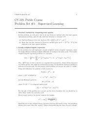
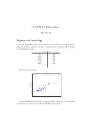
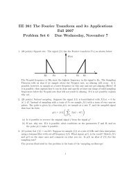
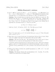
esults in the following error:??? Error using ==> cvx.geDisciplined convex programming error:The left-hand side of a ">=" inequality must be concave.The specifics of the construction rules are discussed in more detail in §4 below. Theserules are relatively intuitive if you know the basics of convex analysis and convexoptimization.2.5 An optimal trade-off curveFor our final example in this section, let us show how traditional Matlab code andcvx specifications can be mixed to form and solve multiple optimization problems.The following code solves the problem of minimizing ‖Ax − b‖ 2 + γ‖x‖ 1 , for a logarithmicallyspaced vector of (positive) values of γ. This gives us points on the optimaltrade-off curve between ‖Ax − b‖ 2 and ‖x‖ 1 . An example of this curve is given inFigure 1.268 gamma = logspace( -2, 2, 20 );269 l2norm = zeros(size(gamma));270 l1norm = zeros(size(gamma));271 fprintf( 1, ’ gamma norm(x,1) norm(A*x-b)\n’ );272 fprintf( 1, ’---------------------------------------\n’ );273 for k = 1:length(gamma),274 fprintf( 1, ’%8.4e’, gamma(k) );275 cvx_begin276 variable x(n);277 minimize( norm(A*x-b)+gamma(k)*norm(x,1) );278 cvx_end279 l1norm(k) = norm(x,1);280 l2norm(k) = norm(A*x-b);281 fprintf( 1, ’ %8.4e %8.4e\n’, l1norm(k), l2norm(k) );282 end283 plot( l1norm, l2norm );284 xlabel( ’norm(x,1)’ );285 ylabel( ’norm(A*x-b)’ );286 gridLine 277 of this code segment illustrates one of the construction rules to be discussedin §4 below. A basic principle of convex analysis is that a convex functioncan be multiplied by a nonnegative scalar, or added to another convex function, andthe result is then convex. cvx recognizes such combinations and allows them to beused anywhere a simple convex function can be—such as an objective function to beminimized, or on the appropriate side of an inequality constraint. So in our example,the expression15

3.63.43.2norm(A*x−b)32.82.62.42.220 0.5 1 1.5 2 2.5 3 3.5norm(x,1)Figure 1: An example trade-off curve from the quickstart demo, lines 268-286.norm(A*x-b)+gamma(k)*norm(x,1)on line 277 is recognized as convex by cvx, as long as gamma(k) is positive or zero. Ifgamma(k) were negative, then this expression becomes the sum of a convex term anda concave term, which causes cvx to generate the following error:??? Error using ==> cvx.plusDisciplined convex programming error:Addition of convex and concave terms is forbidden.16

3 The basics3.1 Data types for variablesAs mentioned above, all variables must be declared using the variable command(or the variables command; see below) before they can be used in constraints or anobjective function.Variables can be real or complex; and scalar, vector, matrix, or n-dimensionalarrays. In addition, matrices can have structure as well, such as symmetry or bandedness.The structure of a variable is given by supplying a list of descriptive keywordsafter the name and size of the variable. For example, the code segmentvariable w(50) complex;variable X(20,10);variable Y(50,50) symmetric;variable Z(100,100) hermitian toeplitz;(inside a cvx specification) declares that w is a complex 50-element vector variable, Xis a real 20×10 matrix variable, Y is a real 50×50 symmetric matrix variable, andZisa complex 100 ×100 Hermitian Toeplitz matrix variable. The structure keywords canbe applied to n-dimensional arrays as well: each 2-dimensional “slice” of the array isgiven the stated structure. The currently supported structure keywords are:banded(lb,ub) complex diagonal hankel hermitian lower_bidiagonallower_hessenberg lower_triangular scaled_identity skew_symmetricsymmetric toeplitz tridiagonal upper_bidiagonal upper_hankelupper_hessenberg upper_triangularWith a couple of exceptions, the structure keywords are self-explanatory:• banded(lb,ub): the matrix is banded with a lower bandwidth lb and an upperbandwidth ub. If both lb and ub are zero, then a diagonal matrix results. ubcan be omitted, in which case it is set equal to lb. For example, banded(1,1)(or banded(1)) is a tridiagonal matrix.• scaled_identity: the matrix is a (variable) multiple of the identity matrix.This is the same as declaring it to be diagonal and Toeplitz.• upper_hankel: The matrix is Hankel (i.e., constant along antidiagonals), andzero below the central antidiagonal, i.e., for i + j > n + 1.When multiple keywords are supplied, the resulting matrix structure is determinedby intersection; if the keywords conflict, then an error will result.A variable statement can be used to declare only a single variable, which canbe a bit inconvenient if you have a lot of variables to declare. For this reason, thevariables statement is provided which allows you to declare multiple variables; i.e.,variables x1 x2 x3 y1(10) y2(10,10,10);The one limitation of the variables command is that it cannot declare complex orstructured arrays (e.g., symmetric, etc.). These must be declared one at a time, usingthe singular variable command.17

3.2 Objective functionsDeclaring an objective function requires the use of the minimize or maximize function,as appropriate. The objective function in a call to minimize must be convex;the objective function in a call to maximize must be concave. At most one objectivefunction may be declared in a given cvx specification, and the objective function musthave a scalar value. (For the only exception to this rule, see the section on definingnew functions in §5).If no objective function is specified, the problem is interpreted as a feasibilityproblem, which is the same as performing a minimization with the objective functionset to zero. In this case, cvx_optval is either 0, if a feasible point is found, or +Inf,if the constraints are not feasible.3.3 ConstraintsThe following constraint types are supported in cvx:• Equality == constraints, where both the left- and right-hand sides are affinefunctions of the optimization variables.• Less-than =, > constraints, where the left-hand expression is concave, andthe right-hand expression is convex.In cvx, the strict inequalities < and > are accepted, but interpreted as the associatednonstrict inequalities, =, respectively. We encourage you to use the nonstrictforms =, since they are mathematically correct. (Future versions of cvxmight assign a slightly different meaning to strict inequalities.)These equality and inequality operators work for arrays. When both sides ofthe constraint are arrays of the same size, the constraint is imposed elementwise. Forexample, ifaandbare m×n matrices, then a=0 isinterpreted as mn inequalities: each element of the matrix must be nonnegative.Note also the important distinction between =, which is an assignment, and ==,which imposes an equality constraint (inside a cvx specification); for more on thisdistinction, see §8.4. Also note that the non-equality operator ~= may not be used ina constraint; in any case, such constraints are rarely convex. Inequalities cannot beused if either side is complex.cvx also supports a set membership constraint; see §3.5.18

3.4 FunctionsThe base cvx function library includes a variety of convex, concave, and affine functionswhich accept cvx variables or expressions as arguments. Many are commonMatlab functions such as sum, trace, diag, sqrt, max, and min, re-implemented asneeded to support cvx; others are new functions not found in Matlab. A completelist of the functions in the base library can be found in §B. It’s also possible to addyour own new functions; see §5.An example of a function in the base library is quad_over_lin, which representsthe quadratic-over-linear function, defined as f(x, y) = x T x/y, with domain R n ×R ++ , i.e., x is an arbitrary vector in R n , and y is a positive scalar. (The function alsoaccepts complex x, but we’ll consider real x to keep things simple.) The quadraticover-linearfunction is convex in x and y, and so can be used as an objective, in anappropriate constraint, or in a more complicated expression. We can, for example,minimize the quadratic-over-linear function of (Ax − b, c T x + d) usingminimize( quad_over_lin( A*x-b, c’*x+d ) );inside a cvx specification, assuming x is a vector optimization variable, A is a matrix,b and c are vectors, and d is a scalar. cvx recognizes this objective expression as aconvex function, since it is the composition of a convex function (the quadratic-overlinearfunction) with an affine function.You can also use the function quad_over_lin outside a cvx specification. Inthis case, it just computes its (numerical) value, given (numerical) arguments. It’snot quite the same as the expression ((A*x-b)’*(A*x-b))/(c’*x+d), however. Thisexpression makes sense, and returns a real number, when c T x + d is negative; butquad_over_lin(A*x-b,c’*x+d) returns +Inf if c T x + d ≯ 0.3.5 Setscvx supports the definition and use of convex sets. The base library includes the coneof positive semidefinite n ×n matrices, the second-order or Lorentz cone, and variousnorm balls. A complete list of sets supplied in the base library is given in §B.Unfortunately, the Matlab language does not have a set membership operator,such as x in S, to denote x ∈ S. So in cvx, we use a slightly different syntax torequire that an expression is in a set. To represent a set we use a function thatreturns an unnamed variable that is required to be in the set. Consider, for example,S n +, the cone of symmetric positive semidefinite n × n matrices. In cvx, we representthis by the function semidefinite(n), which returns an unnamed new variable, thatis constrained to be positive semidefinite. To require that the matrix expression Xbe symmetric positive semidefinite, we use the syntax X == semidefinite(n). Theliteral meaning of this is that X is constrained to be equal to some unnamed variable,which is required to be an n × n symmetric positive semidefinite matrix. This is, ofcourse, equivalent to saying that X must be symmetric positive semidefinite.As an example, consider the constraint that a (matrix) variable X is a correlationmatrix, i.e., it is symmetric, has unit diagonal elements, and is positive semidefinite.In cvx we can declare such a variable and impose such constraints using19

variable X(n,n) symmetric;X == semidefinite(n);diag(X) == ones(n,1);The second line here imposes the constraint that X be positive semidefinite. (You canread ‘==’ here as ‘is’, so the second line can be read as ‘X is positive semidefinite’.)The lefthand side of the third line is a vector containing the diagonal elements of X,whose elements we require to be equal to one. Incidentally, cvx allows us to simplifythe third line todiag(X) == 1;because cvx follows the Matlab convention of handling array/scalar comparisons bycomparing each element of the array independently with the scalar.Sets can be combined in affine expressions, and we can constrain an affine expressionto be in a convex set. For example, we can impose constraints of the formA*X*A’-X == B*semidefinite(n)*B’;where X is an n × n symmetric variable matrix, and A and B are n × n constantmatrices. This constraint requires that AXA T − X = BY B T , for some Y ∈ S n + .cvx also supports sets whose elements are ordered lists of quantities. As an example,consider the second-order or Lorentz cone,Q m = { (x, y) ∈ R m × R | ‖x‖ 2 ≤ y } = epi ‖ · ‖ 2 , (2)where epi denotes the epigraph of a function. An element of Q m is an ordered list,with two elements: the first is an m-vector, and the second is a scalar. We can use thiscone to express the simple least-squares problem from §2.1 (in a fairly complicatedway) as follows:minimize ysubject to (Ax − b, y) ∈ Q m (3).cvx uses Matlab’s cell array facility to mimic this notation:cvx_beginvariables x(n) y;minimize( y );subject to{ A*x-b, y } == lorentz(m);cvx_endThe function call lorentz(m) returns an unnamed variable (i.e., a pair consisting ofa vector and a scalar variable), constrained to lie in the Lorentz cone of length m. Sothe constraint in this specification requires that the pair { A*x-b, y } lies in theappropriately-sized Lorentz cone.20

3.6 Dual variablesWhen a disciplined convex program is solved, the associated dual problem is alsosolved. (In this context, the original problem is called the primal problem.) Theoptimal dual variables, each of which is associated with a constraint in the originalproblem, give valuable information about the original problem, such as the sensitivitieswith respect to perturbing the constraints [BV04, Ch.5]. To get access to theoptimal dual variables in cvx, you simply declare them, and associate them with theconstraints. Consider, for example, the LPminimize c T xsubject to Ax ≼ b,with variable x ∈ R n , and m inequality constraints. The dual of this problem ismaximize −b T ysubject to c + A T y = 0y ≽ 0,where the dual variable y is associated with the inequality constraint Ax ≼ b in theoriginal LP. To represent the primal problem and this dual variable in cvx, we usethe following syntax:The linen = size(A,2);cvx_beginvariable x(n);dual variable y;minimize( c’ * x );subject toy : A * x

It is not necessary to place the dual variable on the left side of the constraint; forexample, the line above can also be written in this way:A * x = A * x : y;yields an identical result. For equality constraints, on the other hand, swapping theleft- and right- hand sides of an equality constraint will negate the optimal value ofthe dual variable.After the cvx_end statement is processed, and assuming the optimization wassuccessful, cvx assigns numerical values to x and y—the optimal primal and dualvariable values, respectively. Optimal primal and dual variables for this LP mustsatisfy the complementary slackness conditionsYou can check this in Matlab with the liney .* (b-A*x)y i (b − Ax) i = 0, i = 1, . . ., m. (4)which prints out the products of the entries of y and b-A*x, which should be nearlyzero. This line must be executed after the cvx_end command (which assigns numericalvalues to x and y); it will generate an error if it is executed inside the cvxspecification, where y and b-A*x are still just abstract expressions.If the optimization is not successful, because either the problem is infeasible orunbounded, then x and y will have different values. In the unbounded case, x willcontain an unbounded direction; i.e., a point x satisfyingc T x = −1, Ax ≼ 0, (5)and y will be filled with NaN values, reflecting the fact that the dual problem isinfeasible. In the infeasible case, x is filled with NaN values, while y contains anunbounded dual direction; i.e., a point y satisfyingb T y = −1, A T y = 0, y ≽ 0 (6)Of course, the precise interpretation of primal and dual points and/or directionsdepends on the structure of the problem. See references such as [BV04] for more onthe interpretation of dual information.cvx also supports the declaration of indexed dual variables. These prove usefulwhen the number of constraints in a model (and, therefore, the number of dualvariables) depends upon the parameters themselves. For more information on indexeddual variables, see §8.5.22

3.7 Expression holdersSometimes it is useful to store a cvx expression into a Matlab variable for future use.For instance, consider the following cvx script:variables x yz = 2 * x - y;square( z )

cvx will accept this construction without error. You can then use the concave expressionsx(1), ..., x(10) in any appropriate ways; for example, you could maximizex(10).The differences between a variable object and an expression object are quitesignificant. A variable object holds an optimization variable, and cannot be overwrittenor assigned in the cvx specification. (After solving the problem, however, cvxwill overwrite optimization variables with optimal values.) An expression object, onthe other hand, is initialized to zero, and should be thought of as a temporary placeto store cvx expressions; it can be assigned to, freely re-assigned, and overwritten ina cvx specification.Of course, as our first example shows, it is not always necessary to declare anexpression holder before it is created or used. But doing so provides an extra measureof clarity to models, so we strongly recommend it.24

4 The DCP rulesetcvx enforces the conventions dictated by the disciplined convex programming ruleset,or DCP ruleset for short. cvx will issue an error message whenever it encountersa violation of any of the rules, so it is important to understand them before beginningto build models. The rules are drawn from basic principles of convex analysis,and are easy to learn, once you’ve had an exposure to convex analysis and convexoptimization.The DCP ruleset is a set of sufficient, but not necessary, conditions for convexity.So it is possible to construct expressions that violate the ruleset but are in factconvex. As an example consider the entropy function, − ∑ ni=1 x i log x i , defined forx > 0, which is concave. If it is expressed as- sum( x .* log( x ) )cvx will reject it, because its concavity does not follow from any of the compositionrules. (Specifically, it violates the no-product rule described in §4.4.) Problemsinvolving entropy, however, can be solved, by explicitly using the entropy function,sum(entr( x ))which is in the base cvx library, and thus recognized as concave by cvx. If a convex(or concave) function is not recognized as convex or concave by cvx, it can be addedas a new atom; see §5.As another example consider the function √ x 2 + 1 = ‖[x 1]‖ 2 , which is convex. Ifit is written asnorm([x 1])(assuming x is a scalar variable or affine expression) it will be recognized by cvxas a convex expression, and therefore can be used in (appropriate) constraints andobjectives. But if it is written assqrt(x^2+1)cvx will reject it, since convexity of this function does not follow from the cvx ruleset.4.1 A taxonomy of curvatureIn disciplined convex programming, a scalar expression is classified by its curvature.There are four categories of curvature: constant, affine, convex, and concave. For afunction f : R n → R defined on all R n , the categories have the following meanings:constant: f(αx + (1 − α)y)= f(x) ∀x, y ∈ R n , α ∈ Raffine: f(αx + (1 − α)y)= αf(x) + (1 − α)f(y) ∀x, y ∈ R n , α ∈ Rconvex: f(αx + (1 − α)y) ≤ αf(x) + (1 − α)f(y) ∀x, y ∈ R n , α ∈ [0, 1]concave: f(αx + (1 − α)y) ≥ αf(x) + (1 − α)f(y) ∀x, y ∈ R n , α ∈ [0, 1]25

Of course, there is significant overlap in these categories. For example, constantexpressions are also affine, and (real) affine expressions are both convex and concave.Convex and concave expressions are real by definition. Complex constant andaffine expressions can be constructed, but their usage is more limited; for example,they cannot appear as the left- or right-hand side of an inequality constraint.4.2 Top-level rulescvx supports three different types of disciplined convex programs:• A minimization problem, consisting of a convex objective function and zero ormore constraints.• A maximization problem, consisting of a concave objective function and zero ormore constraints.• A feasibility problem, consisting of one or more constraints.4.3 ConstraintsThree types of constraints may be specified in disciplined convex programs:• An equality constraint, constructed using ==, where both sides are affine.• A less-than inequality constraint, using either , where the left side isconcave and the right side is convex.Non-equality constraints, constructed using ~=, are never allowed. (Such constraintsare not convex.)One or both sides of an equality constraint may be complex; inequality constraints,on the other hand, must be real. A complex equality constraint is equivalent to tworeal equality constraints, one for the real part and one for the imaginary part. Anequality constraint with a real side and a complex side has the effect of constrainingthe imaginary part of the complex side to be zero.As discussed in §3.5 above, cvx enforces set membership constraints (e.g., x ∈ S)using equality constraints. The rule that both sides of an equality constraint mustbe affine applies to set membership constraints as well. In fact, the returned value ofset atoms like semidefinite() and lorentz() is affine, so it is sufficient to simplyverify the remaining portion of the set membership constraint. For composite valueslike { x, y }, each element must be affine.In this version, strict inequalities are interpreted identically to nonstrictinequalities >=,

4.4 Expression rulesSo far, the rules as stated are not particularly restrictive, in that all convex programs(disciplined or otherwise) typically adhere to them. What distinguishes disciplinedconvex programming from more general convex programming are the rules governingthe construction of the expressions used in objective functions and constraints.Disciplined convex programming determines the curvature of scalar expressionsby recursively applying the following rules. While this list may seem long, it is forthe most part an enumeration of basic rules of convex analysis for combining convex,concave, and affine forms: sums, multiplication by scalars, and so forth.• A valid constant expression is– any well-formed Matlab expression that evaluates to a finite value.• A valid affine expression is– a valid constant expression;– a declared variable;– a valid call to a function in the atom library with an affine result;– the sum or difference of affine expressions;– the product of an affine expression and a constant.• A valid convex expression is– a valid constant or affine expression;– a valid call to a function in the atom library with a convex result;– an affine scalar raised to a constant power p ≥ 1, p ≠ 3, 5, 7, 9, ...;– a convex scalar quadratic form (§4.8);– the sum of two or more convex expressions;– the difference between a convex expression and a concave expression;– the product of a convex expression and a nonnegative constant;– the product of a concave expression and a nonpositive constant;– the negation of a concave expression.• A valid concave expression is– a valid constant or affine expression;– a valid call to a function in the atom library with a concave result;– a concave scalar raised to a power p ∈ (0, 1);– a concave scalar quadratic form (§4.8);– the sum of two or more concave expressions;27

– the difference between a concave expression and a convex expression;– the product of a concave expression and a nonnegative constant;– the product of a convex expression and a nonpositive constant;– the negation of a convex expression.If an expression cannot be categorized by this ruleset, it is rejected bycvx. For matrixand array expressions, these rules are applied on an elementwise basis. We note thatthe set of rules listed above is redundant; there are much smaller, equivalent sets ofrules.Of particular note is that these expression rules generally forbid products betweennonconstant expressions, with the exception of scalar quadratic forms (see §4.8 below).For example, the expression x*sqrt(x) happens to be a convex function of x, butits convexity cannot be verified using the cvx ruleset, and so is rejected. (It can beexpressed as x^(3/2) or pow_p(x,3/2), however.) We call this the no-product rule,and paying close attention to it will go a long way to insuring that the expressionsyou construct are valid.4.5 FunctionsIn cvx, functions are categorized in two attributes: curvature (constant, affine, convex,or concave) and monotonicity (nondecreasing, nonincreasing, or nonmonotonic).Curvature determines the conditions under which they can appear in expressions accordingto the expression rules given in §4.4 above. Monotonicity determines howthey can be used in function compositions, as we shall see in §4.6 below.For functions with only one argument, the categorization is straightforward. Someexamples are given in the table below.Function∑Meaning Curvature Monotonicitysum( x )i x i affine nondecreasingabs( x ) |x| convex nonmonotonicsqrt( x ) √ x concave nondecreasingFollowing standard practice in convex analysis, convex functions are interpretedas +∞ when the argument is outside the domain of the function, and concave functionsare interpreted as −∞ when the argument is outside its domain. In otherwords, convex and concave functions in cvx are interpreted as their extended-valuedextensions.This has the effect of automatically constraining the argument of a function to bein the function’s domain. For example, if we form sqrt(x+1) in a cvx specification,where x is a variable, then x will automatically be constrained to be larger than orequal to −1. There is no need to add a separate constraint, x>=-1, to enforce this.Monotonicity of a function is determined in the extended sense, i.e., including thevalues of the argument outside its domain. For example, sqrt(x) is determined to benondecreasing since its value is constant (−∞) for negative values of its argument;then jumps up to 0 for argument zero, and increases for positive values of its argument.28

cvx does not consider a function to be convex or concave if it is so only overa portion of its domain, even if the argument is constrained to lie in one of theseportions. As an example, consider the function 1/x. This function is convex for x > 0,and concave for x < 0. But you can never write 1/x in cvx (unless x is constant),even if you have imposed a constraint such as x>=1, which restricts x to lie in theconvex portion of function 1/x. You can use the cvx function inv_pos(x), definedas 1/x for x > 0 and ∞ otherwise, for the convex portion of 1/x; cvx recognizes thisfunction as convex and nonincreasing. In cvx, you can express the concave portionof 1/x, where x is negative, using -inv_pos(-x), which will be correctly recognizedas concave and nonincreasing.For functions with multiple arguments, curvature is always considered jointly, butmonotonicity can be considered on an argument-by-argument basis. For example,{|x| 2 /y y > 0quad_over_lin( x, y )convex, nonincreasing in y+∞ y ≤ 0is jointly convex in both arguments, but it is monotonic only in its second argument.In addition, some functions are convex, concave, or affine only for a subset of itsarguments. For example, the functionnorm( x, p ) ‖x‖ p (1 ≤ p) convex in x, nonmonotonicis convex only in its first argument. Whenever this function is used in a cvx specification,then, the remaining arguments must be constant, or cvx will issue an errormessage. Such arguments correspond to a function’s parameters in mathematicalterminology; e.g.,f p (x) : R n → R, f p (x) ‖x‖ pSo it seems fitting that we should refer to such arguments as parameters in thiscontext as well. Henceforth, whenever we speak of a cvx function as being convex,concave, or affine, we will assume that its parameters are known and have been givenappropriate, constant values.4.6 CompositionsA basic rule of convex analysis is that convexity is closed under composition with anaffine mapping. This is part of the DCP ruleset as well:• A convex, concave, or affine function may accept an affine expression (of compatiblesize) as an argument. The result is convex, concave, or affine, respectively.For example, consider the function square( x ), which is provided in the cvx atomlibrary. This function squares its argument; i.e., it computes x.*x. (For array arguments,it squares each element independently.) It is in the cvx atom library, andknown to be convex, provided its argument is real. So if x is a real variable ofdimension n, a is a constant n-vector, and b is a constant, the expressionsquare( a’ * x + b )29

is accepted by cvx, which knows that it is convex.The affine composition rule above is a special case of a more sophisticated compositionrule, which we describe now. We consider a function, of known curvature andmonotonicity, that accepts multiple arguments. For convex functions, the rules are:• If the function is nondecreasing in an argument, that argument must be convex.• If the function is nonincreasing in an argument, that argument must be concave.• If the function is neither nondecreasing or nonincreasing in an argument, thatargument must be affine.If each argument of the function satisfies these rules, then the expression is acceptedby cvx, and is classified as convex. Recall that a constant or affine expression isboth convex and concave, so any argument can be affine, including as a special case,constant.The corresponding rules for a concave function are as follows:• If the function is nondecreasing in an argument, that argument must be concave.• If the function is nonincreasing in an argument, that argument must be convex.• If the function is neither nondecreasing or nonincreasing in an argument, thatargument must be affine.In this case, the expression is accepted by cvx, and classified as concave.For more background on these composition rules, see [BV04, §3.2.4]. In fact, withthe exception of scalar quadratic expressions, the entire DCP ruleset can be thoughtof as special cases of these six rules.Let us examine some examples. The maximum function is convex and nondecreasingin every argument, so it can accept any convex expressions as arguments.For example, if x is a vector variable, thenmax( abs( x ) )obeys the first of the six composition rules and is therefore accepted by cvx, andclassified as convex.As another example, consider the sum function, which is both convex and concave(since it is affine), and nondecreasing in each argument. Therefore the expressionssum( square( x ) )sum( sqrt( x ) )are recognized as valid in cvx, and classified as convex and concave, respectively. Thefirst one follows from the first rule for convex functions; and the second one followsfrom the first rule for concave functions.Most people who know basic convex analysis like to think of these examples interms of the more specific rules: a maximum of convex functions is convex, and a sumof convex (concave) functions is convex (concave). But these rules are just special30

cases of the general composition rules above. Some other well known basic rules thatfollow from the general composition rules are: a nonnegative multiple of a convex(concave) function is convex (concave); a nonpositive multiple of a convex (concave)function is concave (convex).Now we consider a more complex example in depth. Suppose x is a vector variable,and A, b, and f are constants with appropriate dimensions. cvx recognizes theexpressionsqrt(f’*x) + min(4,1.3-norm(A*x-b))as concave. Consider the term sqrt(f’*x). cvx recognizes that sqrt is concave andf’*x is affine, so it concludes that sqrt(f’*x) is concave. Now consider the secondterm min(4,1.3-norm(A*x-b)). cvx recognizes that min is concave and nondecreasing,so it can accept concave arguments. cvx recognizes that 1.3-norm(A*x-b) isconcave, since it is the difference of a constant and a convex function. So cvx concludesthat the second term is also concave. The whole expression is then recognizedas concave, since it is the sum of two concave functions.The composition rules are sufficient but not necessary for the classification to becorrect, so some expressions which are in fact convex or concave will fail to satisfythem, and so will be rejected by cvx. For example, if x is a vector variable, theexpressionsqrt( sum( square( x ) ) )is rejected by cvx, because there is no rule governing the composition of a concavenondecreasing function with a convex function. Of course, the workaround is simplein this case: use norm( x ) instead, since norm is in the atom library and known bycvx to be convex.4.7 Monotonicity in nonlinear compositionsMonotonicity is a critical aspect of the rules for nonlinear compositions. This hassome consequences that are not so obvious, as we shall demonstrate here by example.Consider the expressionsquare( square( x ) + 1 )where x is a scalar variable. This expression is in fact convex, since (x 2 + 1) 2 =x 4 + 2x 2 + 1 is convex. But cvx will reject the expression, because the outer squarecannot accept a convex argument. Indeed, the square of a convex function is not, ingeneral, convex: for example, (x 2 − 1) 2 = x 4 − 2x 2 + 1 is not convex.There are several ways to modify the expression above to comply with the ruleset.One way is to write it as x^4 + 2*x^2 + 1, which cvx recognizes as convex, sincecvx allows positive even integer powers using the ^ operator. (Note that the sametechnique, applied to the function (x 2 −1) 2 , will fail, since its second term is concave.)Another approach is to use the alternate outer function square_pos, included inthe cvx library, which represents the function (x + ) 2 , where x + = max{0, x}. Obviously,square and square_pos coincide when their arguments are nonnegative. But31

square_pos is nondecreasing, so it can accept a convex argument. Thus, the expressionsquare_pos( square( x ) + 1 )is mathematically equivalent to the rejected version above (since the argument to theouter function is always positive), but it satisfies the DCP ruleset and is thereforeaccepted by cvx.This is the reason several functions in the cvx atom library come in two forms:the “natural” form, and one that is modified in such a way that it is monotonic, andcan therefore be used in compositions. Other such “monotonic extensions” includesum_square_pos and quad_pos_over_lin. If you are implementing a new functionyourself, you might wish to consider if a monotonic extension of that function wouldalso be useful.4.8 Scalar quadratic formsIn its original form described in [Gra04, GBY06], the DCP ruleset forbids even theuse of simple quadratic expressions such as x * x (assuming x is a scalar variable).For practical reasons, we have chosen to make an exception to the ruleset to allow forthe recognition of certain specific quadratic forms that map directly to certain convexquadratic functions (or their concave negatives) in the cvx atom library:conj( x ) .* x is replaced with square( x )y’ * y is replaced with sum_square( y )(A*x-b)’*Q*(Ax-b) is replaced with quad_form( A * x - b, Q )cvx detects the quadratic expressions such as those on the left above, and determineswhether or not they are convex or concave; and if so, translates them to an equivalentfunction call, such as those on the right above.cvx examines each single product of affine expressions, and each single squaringof an affine expression, checking for convexity; it will not check, for example, sumsof products of affine expressions. For example, given scalar variables x and y, theexpressionx ^ 2 + 2 * x * y + y ^2will cause an error incvx, because the second of the three terms2 * x * y, is neitherconvex nor concave. But the equivalent expressions( x + y ) ^ 2( x + y ) * ( x + y )will be accepted. cvx actually completes the square when it comes across a scalarquadratic form, so the form need not be symmetric. For example, if z is a vectorvariable, a, b are constants, and Q is positive definite, then( z + a )’ * Q * ( z + b )32

will be recognized as convex. Once a quadratic form has been verified by cvx, itcan be freely used in any way that a normal convex or concave expression can be, asdescribed in §4.4.Quadratic forms should actually be used less frequently in disciplined convex programmingthan in a more traditional mathematical programming framework, wherea quadratic form is often a smooth substitute for a nonsmooth form that one trulywishes to use. In cvx, such substitutions are rarely necessary, because of its supportfor nonsmooth functions. For example, the constraintsum( ( A * x - b ) .^ 2 )

5 Adding new functions to the cvx atom librarycvx allows new convex and concave functions to be defined and added to the atomlibrary, in two ways, described in this section. The first method is simple, and can(and should) be used by many users of cvx, since it requires only a knowledge of thebasic DCP ruleset. The second method is very powerful, but a bit complicated, andshould be considered an advanced technique, to be attempted only by those who aretruly comfortable with convex analysis, disciplined convex programming, and cvx inits current state.Please do let us know if you have implemented a convex or concave function thatyou think would be useful to other users; we will be happy to incorporate it in afuture release.5.1 New functions via the DCP rulesetThe simplest way to construct a new function that works within cvx is to construct itusing expressions that fully conform to the DCP ruleset. To illustrate this, considerthe convex deadzone function, defined as⎧⎨ 0 |x| ≤ 1f(x) = max{|x| − 1, 0} = x − 1 x > 1⎩−1 − x x < −1To implement this function in cvx, simply create a file deadzone.m containingfunction y = deadzone( x )y = max( abs( x ) - 1, 0 )This function works just as you expect it would outside of cvx—i.e., when its argumentis numerical. But thanks to Matlab’s operator overloading capability, it willalso work within cvx if called with an affine argument. cvx will properly concludethat the function is convex, because all of the operations carried out conform to therules of DCP: abs is recognized as a convex function; we can subtract a constant fromit, and we can take the maximum of the result and 0, which yields a convex function.So we are free to use deadzone anywhere in a cvx specification that we might useabs, for example, because cvx knows that it is a convex function.Let us emphasize that when defining a function this way, the expressions youuse must conform to the DCP ruleset, just as they would if they had been inserteddirectly into a cvx model. For example, if we replace max with min above; e.g.,function y = deadzone_bad( x )y = min( abs( x ) - 1, 0 )then the modified function fails to meet the DCP ruleset. The function will workoutside of a cvx specification, happily computing the value min{|x| − 1, 0} for anumerical argument x. But inside a cvx specification, invoked with a nonconstantargument, it will not work, because it doesn’t follow the DCP composition rules.34

5.2 New functions via partially specified problemsA more advanced method for defining new functions in cvx relies on the followingbasic result of convex analysis. Suppose that S ⊂ R n × R m is a convex set andg : (R n × R m ) → (R ∪ +∞) is a convex function. Thenf : R n → (R ∪ +∞), f(x) inf {g(x, y) | ∃y, (x, y) ∈ S } (7)is also a convex function. (This rule is sometimes called the partial minimizationrule.) We can think of the convex function f as the optimal value of a family ofconvex optimization problems, indexed or parametrized by x,minimize g(x, y)subject to (x, y) ∈ Swith optimization variable y.One special case should be very familar: if m = 1 and g(x, y) y, thenf(x) inf {y | ∃y, (x, y) ∈ S }gives the classic epigraph representation of f:epi f = S + ({0} × R + ) ,where 0 ∈ R n .Incvx you can define a convex function in this very manner, that is, as the optimalvalue of a parameterized family of disciplined convex programs. We call the underlyingconvex program in such cases an incomplete specification—so named becausethe parameters (that is, the function inputs) are unknown when the specification isconstructed. The concept of incomplete specifications can at first seem a bit complicated,but it is very powerful mechanism that allows cvx to support a wide varietyof functions.Let us look at an example to see how this works. Consider the unit-halfwidthHuber penalty function h(x):{x 2 |x| ≤ 1h : R → R, h(x) (8)2|x| − 1 |x| ≥ 1.We can express the Huber function in terms of the following family of convex QPs,parameterized by x:minimize 2v + w 2subject to |x| ≤ v + w(9)w ≤ 1,with scalar variables v and w. The optimal value of this simple QP is equal to theHuber penalty function of x. We note that the objective and constraint functions inthis QP are (jointly) convex in v, w and x.We can implement the Huber penalty function in cvx as follows:35

function cvx_optval = huber( x )cvx_beginvariables w v;minimize( w^2 + 2 * v );subject toabs( x )

function cvx_optval = lambda_min_symm( X )n = size( X, 1 );cvx_beginvariable y;maximize( y );subject toX + X’ - y * eye( n ) == semidefinite( n );cvx_endIf a numeric value ofXis supplied, this function will returnmin(eig(X+X’)) (to withinnumerical tolerances). However, this function can also be used in cvx constraints andobjectives, just like any other concave function in the atom library.There are two practical issues that arise when defining functions using incompletespecifications, both of which we will illustrate using ourhuber example above. First ofall, as written the function works only with scalar values. To apply it (elementwise) toa vector requires that we iterate through the elements in afor loop—a very inefficiententerprise, particularly in cvx. A far better approach is to extend the huber functionto handle vector inputs. This is, in fact, rather simple to do: we simply create amultiobjective version of the problem:function cvx_optval = huber( x )sx = size( x );cvx_beginvariables w( sx ) v( sx );minimize( w .^ 2 + 2 * v );subject toabs( x )

endvariables w( sx ) v( sx );minimize( w .^ 2 + 2 * v );subject toabs( x )

6 Semidefinite programming using cvxThose who are familiar with semidefinite programming (SDP) know that the constraintsthat utilize the set semidefinite(n) in §3.5 above are, in practice, typicallyexpressed using linear matrix inequality (LMI) notation. For example, givenX = X T ∈ R n×n , the constraint X ≽ 0 denotes that X ∈ S n +; that is, that X ispositive semidefinite.cvx provides a special SDP mode which allows this LMI convention to be employedinside cvx models using Matlab’s standard inequality operators >=, Y become X - Y == hermitian_semidefinite(n)X = 1 or 1 >= Y illegalX >= ones(n,n) or ones(n,n) >= Y legalX >= 0 or 0 >= Y legalIn effect, cvx enforces a stricter interpretation of the inequality operators forLMI constraints.39

• Note that LMI constraints enforce symmetry (real or Hermitian, as appropriate)on their inputs. Unlike SDPSOL [WB00], cvx does not extract the symmetricpart for you: you must take care to insure symmetry yourself. Since cvx supportsthe declaration of symmetric matrices, this is reasonably straightforward.If cvx cannot determine that an LMI is symmetric, a warning will be issued.• A dual variable, if supplied, will be applied to the converted equality constraint.It will be given a positive semidefinite value if an optimal point is found.So, for example, thecvx model found in the fileexamples/closest_toeplitz_sdp.m,cvx_beginvariable Z(n,n) hermitian toeplitzdual variable Qminimize( norm( Z - P, ’fro’ ) )Z == hermitian_semidefinite( n ) : Q;cvx_endcan also be written as follows:cvx_begin sdpvariable Z(n,n) hermitian toeplitzdual variable Qminimize( norm( Z - P, ’fro’ ) )Z >= 0 : Q;cvx_endMany other examples in the cvx example library utilize semidefinite constraints; andall of them use SDP mode. To find them, simply search for the text cvx_begin sdpin the examples/ subdirectory tree using your favorite file search tool. One of theseexamples is reproduced in §8.5.Since semidefinite programming is popular, some may wonder why SDP mode isnot the default behavior. The reason for this is that we place a strong emphasison maintaining consistency between Matlab’s native behavior and that of cvx; andthe use of the >=, , < operators to create LMIs represents a deviation fromthat ideal. For example, the expression Z >= 0 in the example above constrainsthe variable Z to be positive semidefinite. But after the model has been solved andZ has been replaced with a numeric value, the expression Z >= 0 will test for theelementwise nonnegativity of Z. To verify that the numeric value of Z is, in fact,positive semidefinite, you must perform a test like min(eig(Z)) >= 0.40

7 Geometric programming using cvxGeometric programs (GPs) are special mathematical programs that can be convertedto convex form using a change of variables. The convex form of GPs can be expressedas DCPs, but cvx also provides a special mode that allows a GP to be specified inits native form. cvx will automatically perform the necessary conversion, computea numerical solution, and translate the results back to the original problem. For atutorial on geometric programming, we refer the reader to [BKVH05].To utilize GP mode, you must begin your cvx specification with the commandcvx_begin gp or cvx_begin GP instead of simply cvx_begin. For example, thefollowing code, found in the example library at gp/max_volume_box.m, determinesthe maximum volume box subject to various area and ratio constraints:cvx_begin gpvariables w h dmaximize( w * h * d )subject to2*(h*w+h*d)

• A feasibility problem, consisting of one or more constraints.The asymmetry between minimizations and maximizations—specifically, that onlymonomial objectives are allowed in the latter—is an unavoidable artifact of the geometryof GPs and GGPs.7.2 ConstraintsThree types of constraints may be specified in geometric programs:• An equality constraint, consrtucted using ==, where both sides are monomials.• A less-than inequality constraint =, > where the left side is a monomial andthe right side is a generalized posynomial.As with DCPs, non-equality constraints are not permitted.7.3 ExpressionsThe basic building blocks of generalized geometric programming are monomials,posynomials, and generalized posynomials. A valid monomial is• a declared variable;• the product of two or more monomials;• the ratio of two monomials;• a monomial raised to a real power; or• a call to one of the following functions with monomial arguments: prod,cumprod,geo_mean, sqrt.A valid posynomial expression is• a valid monomial;• the sum of two or more posynomials;• the product of two or more posynomials;• the ratio of a posynomial and a monomial;• a posynomial raised to a positive integral power; or• a call to one of the following functions with posynomial arguments: sum,cumsum,mean, prod, cumprod.42

A valid generalized posynomial expression is• a valid posynomial;• the sum of two or more generalized posynomials;• the product of two or more generalized posynomials;• the ratio of a generalized posynomial and a monomial;• a generalized posynomial raised to a positive real power; or• a call to one of the following functions with arguments that are generalizedposynomials: sum, cumsum, mean, prod, cumprod, geo_mean, sqrt, norm,sum_largest, norm_largest.It is entirely possible to create and manipulate arrays of monomials, posynomials,and/or generalized posynomials in cvx, in which case these rules extend in an obviousmanner. For example, the product of two monomial matrices produces eithera posynomial matrix or a monomial matrix, depending upon the structure of saidmatrices.43

8 Advanced topicsIn this section we describe a number of the more advanced capabilities of cvx. Werecommend that you skip this section at first, until you are comfortable with the basiccapabilities described above.8.1 Solver selectioncvx currently supports two solvers: SeDuMi and SDPT3 (the default). To selectSeDuMi as your default solver, simply type12 cvx_solver sedumiat the command line, outside of a cvx model. To revert to SDPT3, type13 cvx_solver sdpt3To see which solver is currently selected, simply type14 cvx_solverWe have found that SDPT3 is much more reliable for problems that use second-ordercones, which include problems involving absolute values, quadratics, power functions,and norms. SDPT3 is currently in very active development; so if you encounter aproblem that SDPT3 cannot solve but SeDuMi can, please send us a bug report andwe will forward the results to the authors of SDPT3.8.2 Controlling solver precisionNumerical methods for convex optimization are not exact; they compute their resultsto within a predefined numerical precision or tolerance. The precision chosen by defaultin cvx, which in turn is inherited from the defaults chosen by its solver SeDuMi,should be entirely acceptable for most applications. Nevertheless, you may wish totighten or relax that precision in some applications.There are several ways to call the cvx_precision command. If you call it with noarguments, it simply returns a two-element vector of the current precision settings.The first element in that vector is the standard precision; the precision the solvermust obtain to returnSolved, Unbounded, orInfeasible. The second element in thevector is the “reduced” precision, the precision that the solver must achieve in orderto return Solved/Inaccurate, Unbounded/Inaccurate, Infeasible/Inaccurate.Calling cvx_precision with an argument allows you to actually change the precisionlevel. One way is to supply a string as an argument, either in command modeor function mode, chosen from one of five values:• cvx_precision low: standard = reduced = ǫ 1/4 ≈ 1.2 × 10 −4 .• cvx_precision medium: standard = ǫ 3/8 ≈ 1.3 × 10 −6 , reduced = ǫ 1/4 .44

• cvx_precision default: standard = ǫ 1/2 ≈ 1.5 × 10 −8 , reduced = ǫ 1/4 .• cvx_precision high: standard = ǫ 3/4 ≈ 1.1 × 10 −11 , reduced = ǫ 3/8 .• cvx_precision best: standard = 0, “reduced” = ǫ 1/2 (see below).In function mode, these calls look like cvx_precision(’low’), etc. The best precisionsetting is special: it instructs the solver to continue until it is completely unableto make progress. Then, as long as it reaches at least the “reduced” precision ofǫ 1/2 , it may claim a successful solution; otherwise, it returns a cvx_status value ofFailed. An Inaccurate status value is not possible in best mode (nor, for thatmatter, in low mode, which sets the standard and reduced precisions to be identical).The cvx_precision command can also be called with either a scalar or a lengthtwovector. If you pass it a scalar, it will assume that as the standard precision, andit will compute a default reduced precision value for you. Roughly speaking, thatreduced precision will be the square root of the standard precision, with some boundsimposed to make sure that it stays reasonable. If you supply a vector of values, thenthe smallest value will be chosen as the standard precision, and the larger value asthe reduced precision.The cvx_precision command can be used either within a cvx model or outsideof it; and its behavior differs in each case. If you call it from within a model, e.g.,cvx_begincvx_precision high...cvx_endthen the setting you choose will apply only until cvx_end is reached. If you call itoutside a model, e.g.,cvx_precision highcvx_begin...cvx_endthen the setting you choose will apply globally; that is, to any subsequent modelsthat are created and solved. The local approach should be preferred in an applicationwhere multiple models are constructed and solved at different levels of precision.If you call cvx_precision in function mode, either with a string or a numericvalue, it will return as its output the previous precision vector—the same result youwould obtain if you called it with no arguments. This may seem confusing at first,but this is done so that you can save the previous value in a variable, and restore itat the end of your calcuations; e.g.,cvxp = cvx_precision( ’high’ );cvx_begin...cvx_endcvx_precision( cvxp );45

This is considered good coding etiquette in a larger application where multiple cvxmodels at multiple precision levels may be employed. Of course, a simpler but equallycourteous approach is to call cvx_precision within the cvx model, as describedabove, so that its effect lasts only for that model.8.3 Miscellaneous cvx commands• cvx_problem: typing this within a cvx specification provides a summary of thecurrent problem. Note that this will contain a lot of information that you maynot recognize—cvx performs its conversion to canonical form as the problem isentered, generating extra temporary variables and constraints in the process.• cvx_clear: typing this resets the cvx system, clearing any and all problemsfrom memory, but without erasing any of your numeric data. This is useful ifyou make a mistake and need to start over. But note that in current versionsof cvx, you can simply start another model with cvx_begin, and the previousmodel will be erased (with a warning).• cvx_quiet: typing cvx_quiet(true) suppresses screen output from the solver.Typing cvx_quiet(false) restores the screen output. In each case, it returns alogical value representing the previous state of the quiet flag, so you can restorethat state later if you wish—which is good practice if you wish to share yourcode with others.• cvx_pause: typingcvx_pause(true) causescvx to pause and wait for keyboardinput before and after the solver is called. Useful primarily for demo purposes.Typing cvx_pause(false) resets the behavior. In each case, it returns a logicalvalue representing the previous state of the pause flag, so you can restore thatstate later if you wish.• cvx_where: returns the directory where thecvx distribution has been installed—assuming that the Matlab path has been set to include that distribution. Usefulif you want to find certain helpful subdirectories, such as doc, examples, etc.• cvx_version: returns a description of the cvx version number, build number,and hardware platform you are currently using. If you encounter a bug in cvx,please run this function and copy its output into your email message along witha description of your problem.8.4 Assignments versus equality constraintsAnyone who has used the C or Matlab languages for a sufficiently long time understandsthe differences between assignments, which employ a single equals sign =operator, and an equality, which employs the double equal == operator. In cvx, thisdistinction is particularly important; confusing the two operators can have seriousconsequences. Even when the distinction is well understood, there are importantcaveats to using assignments in cvx that we address here as well.46

The consequences of inadvertently using assignments within a cvx specificationcan cause subtle but critical problems. For example, let A, C ∈ R n×n and b ∈ R begiven, and consider the simple SDPminimize Tr(CX)subject to Tr(AX) = bX ≽ 0(14)Suppose that we tried to express this problem in cvx as follows:1 n = 5;2 A = randn(n,n); C = randn(n,n); b = randn;3 cvx_begin4 variable X(n,n) symmetric;5 minimize( trace( C * X ) );6 subject to7 trace( A * X ) == b;8 X = semidefinite(n);9 cvx_endAt first glance, line 8 may look like it constrains X to be positive semidefinite; butit is an assignment, not an equality constraint. So X is actually overwritten with ananonymous, positive semidefinite variable, and the original X is not constrained all!Fortunately, this particular error is easily caught and prevented by cvx. Whencvx_end is reached, cvx examines each declared variable to verify that it still pointsto the variable object it was originally assigned upon declaration. If it does not, itwill issue an error like this:??? Error using ==> cvx_endThe following cvx variable(s) have been overwritten:XThis is often an indication that an equality constraint waswritten with one equals ’=’ instead of two ’==’. The modelmust be rewritten before cvx can proceed.We hope that this check will prevent at least some typographical errors from havingfrustrating consequences in your models.Of course, this single check does not prevent you from using all assignmentsinside your cvx specifications, only those that overwrite formally declared variables.As discussed in §3.7, other kinds of assignments are permitted, and may be genuinelyuseful. But in our view they should be used sparingly. For instance, consider the firstexample from §3.7:variables x yz = 2 * x - y;square( z )

The following alternative formulation, which declares z as a formal variable, is numericallyequivalent:variables x y zz == 2 * x - y;square( z )

dual variables y{n}minimize( ( n - 1 : -1 : 0 ) * diag( X ) );for k = 0 : n-1,sum( diag( X, k ) ) == b( k+1 ) : y{k+1};endX == semidefinite(n);cvx_endThe statementdual variables y{n}allocates a cell array of n dual variables, and stores the result in the Matlab variableZ. The equality constraint in the for loop has been augmented with a referenceto y{k+1}, so that each constraint is assigned a separate dual variable. When thecvx_end command is issued, cvx will compute the optimal values of these dual variables,and deposit them into an n-element cell array y.This example admittedly is a bit simplistic. With a bit of careful arrangement, itis possible to rewrite this model so that the n equality constraints can be combinedinto a single vector constraint, which in turn would require only a single vector dualvariable. 3 For a more complex example that is not amenable to such a simplification,see the fileexamples/cvxbook/Ch07_statistical_estim/cheb.min the cvx distribution. In that problem, each constraint in the for loop is a linearmatrix inequality, not a scalar linear equation; so the indexed dual variables aresymmetric matrices, not scalars.3 Indeed, a future version of cvx will support the use of the Matlab function spdiags, which willreduce the entire for loop to the single constraint spdiags(X,0:n-1)==b.49

A Installation and compatabilitycvx requires Matlab 6.1 or later. 4 Primary cvx development is performed using anIntel-based Mac running Matlab 7.4, with additional development performed on thefollowing platforms and Matlab versions:• Windows (32-bit): Matlab 6.1, 7.4• Linux (32-bit): Matlab 6.1, 7.4• Linux (64-bit): Matlab 7.1, 7.4For purposes of testing and support, we have access to most other versions of Matlabfor Windows, Linux, and Mac (both Intel and PowerPC). The one significantexception is version 7.0.0, so we cannot provide support for it.Version 7.0.0 has exhibited numerical problems for at least one user; the problemswere eliminated by upgrading. We have also identified another issue using cvx withMatlab 7.0.1 and 7.0.4; workarounds are provided in §A.4 below.Precompiled MEX files are included for Windows (32-bit), Linux (32-bit), andIntel Mac OS X. For other platforms, the MEX files will be compiled during thesetup process; see §A.2. For platforms other than those listed above (e.g., Solaris,HPUX), cvx is quite likely to work, but we are unable to provide support.A.1 Basic instructions1. Retrieve the latest version of cvx from http://www.stanford.edu/~boyd/cvx.You can download the package as either a .zip file or a .tar.gz file.2. If you have been running a previous version of cvx, remove it or move it outof the way—say, by renaming it cvx_old—before proceeding. DO NOT allowthe new version of cvx to be unpacked on top of the old.3. Unpack the file anywhere you like; a directory called cvx will be created. Thereis one important exception: do not placecvx in Matlab’s owntoolbox directory.(If your previous installation of cvx was placed there, you’ll need to move itout of there.)4. Start Matlab.5. Change the current directory to the location of cvx. For example, if you unpackedcvx.zipon your Windows machine into the directoryC:\Matlab\personal,then you would typecd C:\Matlab\personal\cvx4 Previous versions of this manual stated that cvx required Matlab 6.0 or later; we have sincediscovered that version 6.0 is not sufficient.50

at the Matlab command prompt. Alternatively, if you unpacked cvx.tar.gzinto the directory ~/matlab on a Linux machine, then you would typecd ~/matlab/cvxat the Matlab command prompt.6. Type the commandcvx_setupat the Matlab prompt. This does two things: it sets the Matlab search pathso it can find all of the cvx program files, and it runs a simple test problem toverify the installation. On some platforms, it compiles MEX files as well (see§A.2 below). If all goes well, the command will output the lineNo errors! cvx has been successfully installed.(among others). If this message is not displayed, or any warnings or errors aregenerated, then there is a problem with the cvx installation. Try installing thepackage again; and if that fails, send us a bug report and tell us about it.7. If you plan to use cvx regularly, you will need to save the current Matlab pathfor subsequent Matlab sessions. Follow the instructions provided by cvx_setupto accomplish that.A.2 MEX file compilationPrecompiled MEX files are provided only for a handful of platforms; for others, theymust be compiled by the user. The cvx_setup script will automatically detect theabsence of compiled MEX files and compile them for SeDuMi, SDPT3, and cvx.However, cvx_setup will succeed only if the MEX system is configured properly onyour machine. If you have compiled MEX files before, this is likely the case; otherwise,run the commandmex -setupat the Matlab prompt and answer the questions that follow. If necessary, consultdocumentation for Matlab for details on this process.A.3 About SeDuMi and SDPT3The cvx distribution includes copies of the solvers SeDuMi and SDPT3 in the directoriescvx/sedumi and cvx/sdpt3, respectively. We strongly recommend that youuse our versions of these solvers, and remove any other versions that you have in yourMatlab path. The version of SeDuMi provided with cvx incorporates some bug fixesand a slight modification that is not currently found in versions available from theauthors. This is not the case with SDPT3; however, the author of SDPT3 frequently51

posts bug fixes to the software without updating the version number (currently 4.0beta). Therefore, it is important to be sure that any newer version of SDPT3 thatyou might wish to use was downloaded after you obtained cvx.A.4 A Matlab 7.0 issueThe techniques that cvx use to embed a new modeling language inside Matlab seemto cause some confusion for Matlab 7.0, specifically version 7.0.4 (R14SP2). We arereasonably confident that the issue is due to a bug in Matlab itself. It does not occurin versions 6.5.2 and earlier, or 7.1 and later. It may occur in earlier versions ofMatlab 7.0 as well (R14,R14SP1).The bug is this: in some circumstances, a.m-file containing a cvx model will causean error that looks like this:??? Error: File: thrusters.m Line: 43 Column: 5"p" was previously used as a variable,conflicting with its use here as the name of a function.The file name, line/column numbers, and variable name may differ, but the errormessage remains the same. The example that produced this particular error is asimple inequality constraintp >= -5;where p is a cvx variable previously declared with a variable statement. Interestingly,a different inequality constraintu >= 0in the same model causes no complaint. So we cannot offer you a precise set ofcircumstances that cause the error.Fortunately, the workaround is very simple: simply remove all of the extra spacein the constraint. In this example, changing the constraint top>=-5;eliminates the error. You may still indent the constraint as you wish—just removethe intermediate spaces.We have no idea why this workaround works, but it does—reliably.52

B Operators, functions, and setsB.1 Basic operators and linear functionsMatlab’s standard arithmetic operations for addition +, subtraction -, multiplication* .*, division / \ ./ ./ .\, and exponentiation ^ .^ have been overloaded to workin cvx whenever appropriate—that is, whenever their use is consistent with bothstandard mathematical and Matlab conventions and the DCP ruleset. For example:• Two cvx expressions can be added together if they are of the same dimension(or one is scalar) and have the same curvature (i.e., both are convex, concave,or affine).• A cvx expression can be multiplied or divided by a scalar constant. If theconstant is positive, the curvature is preserved; if it is negative, curvature isreversed.• An affine column vector cvx expression can be multiplied by a constant matrixof appropriate dimensions; or it can be left-divided by a non-singular constantmatrix of appropriate dimension.Numerious other combinations are possible, of course. For example, the use of theexponentiation operators ^ .^ are somewhat limited; see §B.2 below.Matlab’s basic matrix manipulation and arithmetic operations have been extendedto work with cvx expressions as well, including:• Concatenation: [ A, B ; C, D ]• Indexing: x(n+1:end), X([3,4],:), etc.• Indexed assignment, including deletion: y(2:4) = 1, Z(1:4,:) = [], etc.• Transpose and conjugate transpose: Z.’, y’A number of Matlab’s basic functions have been extended to work with cvx expressionsas well:conj conv cumsum diag dot find fliplr flipud flipdim horzcathankel ipermute kron permute repmat reshape rot90 sparse sumtrace tril triu toeplitz vertcatMost should behave identically with cvx expressions as they do with numeric expressions.Those that perform some sort of summation, such as cumsum, sum, ormultiplication, such as conv, dot or kron, can only be used in accordance with thedisciplined convex programming rules. For example, kron(X,Y) is valid only if eitherX or Y is constant; and trace(Z) is valid only if the elements along the diagonal havethe same curvature.53

B.2 Nonlinear functionsWhat follows are two lists of nonlinear functions supported by cvx: first, a list ofstandard Matlab functions extended to work with cvx; and second, a list of newfunctions created specifically for use in cvx.In some cases, limitations of the underlying solvers place certain restrictions orcaveats on their use:• Functions marked with a dagger (†) are not supported natively by the solversthat cvx uses. They are handled using a successive approximation method,which makes multiple calls to the underlying solver, achieving the same finalprecision. (See §D.1 for details.) If you use one of these functions, you will bewarned that successive approximation will be used.• Functions involving powers (e.g.,x^p) and p-norms (e.g.,norm(x,p)) are markedwith a star (⋆). cvx represents these functions exactly when p is a rational number.For irrational values of p, a nearby rational is selected using Matlab’s ratfunction. See §D.2 for details.B.2.1 Built-in functions• abs: absolute value for real and complex arrays. Convex.• † exp: exponential. Convex and nondecreasing.• † log: logarithm. Concave and nondecreasing.• max: maximum. Convex and nondecreasing.• min: minimum. Concave and nondecreasing.• ⋆ norm: norms for real and complex vectors and matrices. Convex. The oneargumentversion norm(x) computes the 2-norm for vectors and induced 2-norm(maximum singular value) for matrices. The two-argument version norm(x,p)is supported as follows:– For vectors, all p ≥ 1 are accepted, but see Appendix D.2 for more detailsabout how cvx handles values other than 1, 2, and Inf.– For matrices, p must be 1, 2, Inf, or ’Fro’.• polyval: polynomial evaluation. polyval(p,x), where p is a vector of lengthn, computesp(1) * x.^(n-1) + p(2) * x.^(n-2) + ... + p(n-1) * x + p(n)This function can be used in cvx in two ways:54

– If p is a variable and x is a constant, then polyval(x,p) computes a linearcombination of the elements of p. The combination must satisfy the DCPrules for addition and scaling.– If p is a constant and x is a variable, then polyval(x,p) constructs apolynomial function of the variable x. The polynomial must be affine,convex, or concave, and x must be real and affine.• ⋆ power: x^p and x.^p, where x is a real variable and and p is a real constant.For x^p, x and p must be scalars. Only those values of p which can reasonablyand unambiguously interpreted as convex or concave are accepted:– p = 0. Constant. x.^p is identically 1.– 0 < p < 1. Concave. The argument x must be concave (or affine), and isimplicitly constrained to be nonnegative.– p = 1. Affine. x.^p is then x.– p ∈ {2, 4, 6, 8, ...}. Convex. Argument x must be affine.– p > 1, p ∉ {2, 3, 4, 5, ...}. Convex. Argument x must be affine, and isimplicitly constrained to be nonnegative.Negative and odd integral values of p are not permitted, but see the functionspow_p, pow_pos, and pow_abs in the next section for useful alternatives.• † power: p.^x and p^x, where p is a real constant and x is a real variable. Forp^x, p and x must be scalars. Valid values of p include:– p ∈ {0, 1}. Constant.– 0 < p < 1. Convex and nonincreasing; x must be concave.– p > 1. Convex and nondecreasing; x must be convex.Negative values of p are not permitted.• sqrt: square root. Implicitly constrains its argument to be nonnegative. Concaveand nondecreasing.B.2.2 New nonlinear functionsEven though these functions were developed specifically for cvx, they work outsideof a cvx specification as well, when supplied with numeric arguments.• berhu(x,M): The reversed Huber function (hence, Berhu), defined as |x| for|x| ≤ M, and (|x| 2 + M 2 )/2M for |x| ≥ M. Convex. If M is omitted, M = 1is assumed; but if supplied, it must be a positive constant. Also callable withthree arguments as berhu(x,M,t), which computes t+t*berhu(x/t,M), usefulfor concomitant scale estimation (see [Owe06]).55

• det_inv: determinant of inverse of a symmetric (or Hermitian) positive definitematrix, (det X −1 ), which is the same as the sum of the inverses of the eigenvalues.When used inside a cvx specification, det_inv constrains the matrix to besymmetric (if real) or Hermitian (if complex) and positive semidefinite. Whenused with numerical arguments, det_inv returns -Inf if these constraints arenot met. Concave.• det_rootn: n-th root of the determinant of a semidefinite matrix, (det X) 1/n .When used inside a cvx specification, det_rootn constrains the matrix to besymmetric (if real) or Hermitian (if complex) and positive semidefinite. Whenused with numerical arguments, det_rootn returns -Inf if these constraintsare not met. Concave.• det_root2n: the 2n-th root of the determinant of a semidefinite matrix; i.e.,det_root2n(X)=sqrt(det_rootn(X)). Concave. Maintained solely for backcompatibilitypurposes.• † entr, the elementwise entropy function: entr(x)=x.*log(x). Concave. Returns-Inf when called with a constant argument that has a negative entry.• geo_mean: the geometric mean of a vector, ( ∏ nk=1 x k) 1/n . When used inside acvx specification, geo_mean constrains the elements of the vector to be nonnegative.When used with numerical arguments, geo_mean returns -Inf if anyelement is negative. Concave and increasing.• huber(x,M), defined as 2M|x|−M 2 for |x| ≥ M, and |x| 2 for |x| ≤ M. Convex.If M is omitted, then M = 1 is assumed; but if it supplied, it must be a positiveconstant. Also callable as huber(x,M,t), which computes t+t*huber(x/t,M),useful for concomitant scale estimation (see [Owe06]).• huber_circ(x,M), the circularly symmetric Huber function, defined as ‖x‖ 2for ‖x‖ 2 ≤ M, and 2M‖x‖ 2 − M 2 for ‖x‖ 2 ≥ M. Same (and implemented) ashuber_pos(norm(x),M). Convex.• huber_pos(x,M). Same as Huber function for nonnegative x; zero for negativex. Convex and nondecreasing.• inv_pos, inverse of the positive portion, 1/ max{x, 0}. Inside cvx specification,imposes constraint that its argument is positive. Outside cvx specification,returns +∞ if x ≤ 0. Convex and decreasing.• †kl_div, elementwise Kullback-Leibler distance,kl_div(x,y)=x.*log(x./y)-x+y,for x, y nonnegative, with x(i) zero whenever y(i) is zero. Convex. Outsidecvx specification, returns +∞ if arguments aren’t in the domain.• lambda_max: maximum eigenvalue of a real symmetric or complex Hermitianmatrix. Inside cvx, imposes constraint that its argument is symmetric (if real)or Hermitian (if complex). Convex.56

• lambda_min: minimum eigenvalue of a real symmetric or complex Hermitianmatrix. Inside cvx, imposes constraint that its argument is symmetric (if real)or Hermitian (if complex). Concave.• log_det: log of determinant of a positive definite matrix, log det(X). Whenused inside a cvx specification, log_det constrains its argument to be symmetric(if real) or Hermitian (if complex) and positive definite. With numericalargument, log_det returns -Inf if these constraints are not met. Concave.• ⋆ log_norm_cdf(x): logarithm of cumulative distribution function of standardnormal random variable. Concave and increasing. The current implementationis a fairly crude SDP-representable approximation, with modest accuracy overthe interval [−4, 4]; we intend to replace it with a much better approximationat some point.• † log_sum_exp(x): the logarithm of the sum of the elementwise exponentialsof x. Convex and nondecreasing. This is used internally in expert GP mode,but can also be used in standard DCPs.• logsumexp_sdp: a polynomial approximation to the log-sum-exp function withglobal absolute accuracy. This approximation is used in default GP mode, butcan also be used in standard DCPs.• matrix_frac(x,Y): matrix fractional function, x T Y −1 x. In cvx, imposes constraintthat Y is symmetric (or Hermitian) and positive definite; outside cvx,returns +∞ unless Y = Y T ≻ 0. Convex.• norm_largest( x, k ), for real and complex vectors, returns the sum of thelargest k magnitudes in the vector x. Convex.• norm_nuc(X), is the sum of the singular values of a real or complex matrix X.(This is the dual of the usual spectral matrix norm, i.e., the largest singularvalue.) Convex.• ⋆ norms( x, p, dim ) and norms_largest( x, k, dim ). Computes vectornorms along a specified dimension of a matrix or N-d array. Useful for sum-ofnormsand max-of-norms problems. Convex.• poly_env( p, x ). Computes the value of the convex or concave envelopeof the polynomial described by p (in the polyval sense). p must be a realconstant vector whose length n is 0, 1, 2, 3, or some other odd length; and xmust be real and affine. The sign of the first nonzero element of p determineswhether a convex (positive) or concave (negative) envelope is constructed. Forexample, consider the function p(x) (x 2 − 1) 2 = x 4 − 2x 2 + 1, depicted alongwith its convex envelope in Figure 2. The two coincide when |x| ≥ 1, butdeviate when |x| < 1. Attempting to call polyval([1,0,2,0,1],x) in a cvxmodel would yield an error, but a call to poly_env([1,0,2,0,1],x) yields a57

1.6 (x 2 −1) 2envelope1.41.210.80.60.40.20−0.2−1.5 −1 −0.5 0 0.5 1 1.5Figure 2: The polynomial function p(x) = x 4 − 2x 2 + 1 and its convex envelope.valid representation of the envelope. For convex or concave polynomials, thisfunction produces the same result as polyval.• pos: max{x, 0}, for real x. Convex and increasing.• ⋆ pow_abs(x,p): |x| p for x ∈ R or x ∈ C and p ≥ 1. Convex. If p is irrational,a nearby rational value is chosen; see Appendix D.2 for details.• ⋆ pow_pos(x,p): max{x, 0} p for x ∈ R and p ≥ 1. Convex and nondecreasing.If p is irrational, a nearby rational value is chosen; see Appendix D.2 for details.• ⋆ pow_p(x,p), for x ∈ R and real constant p computes nonnegative convex andconcave branches of the power function:{p ≤ 0 : f p (x)x p x > 0+∞ x ≤ 0{convex, nonincreasing0

• quad_over_lin, x T x/y for x ∈ R n , y > 0; for x ∈ C n , y > 0: x ∗ x/y. In cvxspecification, adds constraint that y > 0. Outside cvx specification, returns+∞ if y ≤ 0. Convex, and decreasing in y.• quad_pos_over_lin: sum_square_pos( x ) / y for x ∈ R n , y > 0. Convex,increasing in x, and decreasing in y.• † rel_entr: Scalar relative entropy: rel_entr(x,y)=x.*log(x/y). Convex.• sigma_max: maximum singular value of real or complex matrix. Same as norm.Convex.• square: x 2 for x ∈ R. Convex.• square_abs: |x| 2 for x ∈ R or x ∈ C.• square_pos: max{x, 0} 2 for x ∈ R. Convex and increasing.• sum_largest(x,k) sum of the largest k values, for real vector x. Convex andincreasing.• sum_smallest(x,k), sum of the smallest k values, i.e., -sum_smallest(-x,k).Concave and decreasing.• sum_square: sum( square( x ) ). Convex.• sum_square_abs: sum( square_abs( x ) ). Convex.• sum_square_pos: sum( square_pos( x ) ); works only for real values. Convexand increasing.• trace_inv(X), trace of the inverse of an SPD matrix X, which is the same asthe sum of the inverses of the eigenvalues. Convex. Outside of cvx, returns+Inf if argument is not positive definite.• trace_sqrtm(X), trace of the matrix squareroot of a positive semidefinite matrixX. which is the same as the sum of the squareroots of the eigenvalues.Concave. Outside of cvx, returns +Inf if argument is not positive semidefinite.B.3 Setscvx currently supports the following sets; in each case, n is a positive integer constant.• nonnegative(n):R n + { x ∈ Rn | x i ≥ 0, i = 1, 2, . . .,n}• simplex(n):R n 1+ {x ∈ Rn | x i ≥ 0, i = 1, 2, . . ., n,∑i x i = 1 }59

• lorentz(n):Q n { (x, y) ∈ R n × R | ‖x‖ 2 ≤ y }• rotated_lorentz(n):Q n r {(x, y, z) ∈ Rn × R × R | ‖x‖ 2 ≤ yz, y, z ≥ 0 }• complex_lorentz(n):Q n c {(x, y) ∈ Cn × R | ‖x‖ 2 ≤ y }• rotated_complex_lorentz(n):Q n rc {(x, y, z) ∈ Cn × R × R | ‖x‖ 2 ≤ yz, y, z ≥ 0 }• semidefinite(n):S n + { X ∈ R n×n | X = X T , X ≽ 0 }• hermitian_semidefinite(n):H n + { Z ∈ C n×n | Z = Z H , X ≽ 0 }• nonneg_poly_coeffs(n): The cone of all coefficients of nonnegative polynomialsof degree n; n must be even:{}n∑P +,n p ∈ R n+1 | p i+1 x n−i ≥ 0 ∀x ∈ Ri=0• convex_poly_coeffs(n): The cone of all coefficients of convex polynomials ofdegree n; n must be even:{}∑n−2P +,n p ∈ R n+1 | (n − i)(n − i − 1)p i+1 x n−i−2 ≥ 0 ∀x ∈ Ri=0• exponential_cone:E cl { (x, y, z) ∈ R × R × R | y > 0, ye x/y ≤ z }• geo_mean_cone(n):{}n∏G n cl (x, y) ∈ R n × R n × R n | x ≥ 0, ( x i ) 1/n ≥ yi=160

C cvx status messagesAfter a completecvx specification has been entered and thecvx_end command issued,the solver is called to generate a numerical result. The solver can produce one of fiveexit conditions, which are indicated by the value of the string variable cvx_status.The nominal values of cvx_status, and the resulting values of the other variables,are as follows:• Solved: A complementary (primal and dual) solution has been found. Theprimal and dual variables are replaced with their computed values, and the theoptimal value of the problem is placed in cvx_optval (which, by convention, is0 for feasibility problems).• Unbounded: The problem has been proven to be unbounded below through thediscovery of an unbounded primal direction. This direction is stored in theprimal variables. The value of cvx_optval is set to -Inf for minimizations,and -Inf for maximizations. Feasibility problems by construction cannot beunbounded below.It is important to understand that the unbounded primal direction is very likelynot a feasible point. If a feasible point is required, the problem should be resolvedas a feasibility problem by omitting the objective.• Infeasible: The problem has been proven to be infeasible through the discoveryof an unbounded dual direction. Appropriate components of this directionare stored in the dual variables. The values of the primal variables are filled withNaNs. The value of cvx_optval is set to +Inf for minimizations and feasibilityproblems, and -Inf for maximizations.In some cases, SeDuMi is unable to achieve the numerical certainty it requires to makeone of the above determinations—but is able to draw a weaker conclusion by relaxingthose tolerances somewhat. In such cases, one of the following results is returned:• Inaccurate/Solved: The problem is likely to have a complementary solution.• Inaccurate/Unbounded: The problem is likely to be unbounded.• Inaccurate/Infeasible: The problem is likely to be infeasible.The values of the primal and dual variables, and of cvx_optval, are updated identicallyto the “accurate” cases. Two final results are also possible:• Failed: The solver failed to make sufficient progress towards a solution. Thevalues of cvx_optval and primal and dual variables are filled with NaNs. Thisresult can occur because of numerical problems within SeDuMi, often becausethe problem is particularly “nasty” in some way (e.g., a non-zero duality gap).61

• Overdetermined: The presolver has determined that the problem has moreequality constraints than variables, which means that the coefficient matrixof the equality constraints is singular. In practice, such problems are often,but not always, infeasible. Unfortunately, solvers typically cannot handle suchproblems, so a precise conclusion cannot be reached.The situations that most commonly produce an Overdetermined result are discussedin §D.3 below.62

D Advanced solver topicsD.1 The successive approximation methodPrior to version 1.2, the functions requested most often to be added to the cvxfunction library were those from the exponential family, including exp, log, andvarious entropy functions. Unfortunately, cvx utilizes symmetric primal/dual solversthat simply cannot support those functions natively; and a variety of practical factorshas delayed the use of other types of solvers with cvx.For this reason, we have constructed a successive approximation method thatallows symmetric primal/dual solvers to support the exponential family of functions.The precise nature of the method will be published elsewhere, but we can providea highly simplified description here. First, we construct a global approximation forexp (or log, etc..) which is accurate within a neighborhood of some center pointx 0 . Solving this approximation yields an approximate optimal point ¯x. We shift thecenter point x 0 towards ¯x, construct a new approximation, and solve again. Thisprocess is repeated until |¯x − x 0 | is small enough to conclude that our approximateis accurate enough to represent the original model. Again, this is a highly simplifieddescription of the approach; for instance, we are also monitoring the dual problem aswell to guide our judgements for shifting x 0 and terminating.D.2 Irrational powersIn order to implement power expressions like x p and p-norms ‖x‖ p for 1 < p < ∞, cvxuses an SDP-compatible method described in [AG01], and enhanced by the authorsof cvx. This approach is exact—as long as the exponent p is rational. To determineintegral values p n , p d such that p n /p d = p, cvx uses Matlab’s rat function with itsdefault tolerance of 10 −6 . There is currently no way to change this tolerance. See thedocumentation for rat for more details.The complexity of the SDP implementation depends on roughly on the size of thevalues p n and p d . Let us introduce a more precise measure of this complexity. Forp = 2, a constraint x p ≤ y can be represented with exactly one 2 × 2 LMI:[ ] y xx 2 ≤ y =⇒ ≽ 0.x 1For other values of p = p n /p d , cvx generates a number of 2 ×2 LMIs that depends onboth p n and p d ; we denote this number by k(p n , p d ). (A number of internal variablesand equality constraints are also generated, but we ignore them for this analysis.) Anempirical study has shown that for p = p n /p d > 1, cvx achievesk(p n , p d ) ≤ log 2 p n + α(p n ),where the α(p n ) term grows very slowly compared to the log 2 term. Indeed, forp n ≤ 4096, we have verified that α(p n ) is usually 1 or 2, but occasionally 0 or 3.Similar results are obtained for 0 < p < 1 and p < 0.63

The cost of this SDP representation is relatively small for nearly all useful values ofp. Nevertheless, cvx issues a warning whenever k(p n , p d ) > 10 to insure that the user isnot surprised by any unexpected slowdown. In the event that this threshold does notsuit you, you may change it using the command cvx_power_warning(thresh), wherethresh is the desired cutoff value. Setting the threshold to Inf disables it completely.As with the command cvx_precision, you can place a call to cvx_power_warningwithin a model to change the threshold for a single model; or outside of a modelto make a global change. The command always returns the previous value of thethreshold, so you can save it and restore it upon completion of your model, if you wish.You can query the current value by calling cvx_power_warning with no arguments.D.3 Overdetermined problemsThis status message Overdetermined commonly occurs when structure in a variableor set is not properly recognized. For example, consider the problem of finding thesmallest diagonal addition to a matrix W ∈ R n×n to make it positive semidefinite:minimize Trace Dsubject to W + D ≽ 0D diagonal(16)In cvx, this problem might be expressed as follows:n = size(W,1);cvx_beginvariable D(n,n) diagonal;minimize( trace( D ) );subject toW + D == semidefinite(n);cvx_endIf we apply this specification to the matrix W=randn(5,5), a warning is issued,Warning: Overdetermined equality constraints;problem is likely infeasible.and the variable cvx_status is set to Overdetermined.What has happened here is that the unnamed variable returned by statementsemidefinite(n) is symmetric, but W is fixed and unsymmetric. Thus the problem,as stated, is infeasible. But there are also n 2 equality constraints here, and onlyn + n ∗ (n + 1)/2 unique degrees of freedom—thus the problem is overdetermined.The following modified version of the specification corrects this problem by extractingthe symmetric part of W:n = size(W,1);cvx_beginvariable D(n,n) diagonal;64

minimize( trace( D ) );subject to0.5 * ( W + W’ ) + D == semidefinite(n);cvx_endE AcknowledgementsWe wish to thank the following people for their contributions to the development ofcvx: Toh Kim Chuan, Laurent El Ghaoui, Arpita Ghosh, Siddharth Joshi, JohanLöfberg, Almir Mutapcic, Michael Overton and his students, Art Owen, Rahul Panicker,Imre Polik, Joëlle Skaf, Lieven Vandenberghe, Argyris Zymnis. We are alsograteful to the many students in several universities who have (perhaps unwittingly)served as beta testers by using cvx in their classwork. We thank Igal Sason for catchingmany typos in an earlier version of this document, and generally helping us toimprove its clarity.65

References[AG01]F. Alizadeh and D. Goldfarb. Second-order cone programming. TechnicalReport RRR 51-2001, RUTCOR, Rutgers University, November 2001.Available at http://rutcor.rutgers.edu/pub/rrr/reports2001/51.ps.[BKMR98] A. Brooke, D. Kendrick, A. Meeraus, and R. Raman. GAMS: A User’sGuide. The Scientific Press, South San Francisco, 1998. Available at http://www.gams.com/docs/gams/GAMSUsersGuide.pdf.[BKVH05] S. Boyd, S. J. Kim, L. Vandenberghe, and A. Hassibi. A tutorial ongeometric programming. Optimization and Engineering, 2005. Available athttp://www.stanford.edu/~boyd/gp_tutorial.html.[BV04][Cru02][DV05]S. Boyd and L. Vandenberghe. Convex Optimization. Cambridge UniversityPress, 2004. Available athttp://www.stanford.edu/~boyd/cvxbook.html.C. Crusius. A Parser/Solver for Convex Optimization Problems. PhDthesis, Stanford University, 2002.J. Dahl and L. Vandenberghe. CVXOPT: A Python Package for ConvexOptimization. Available at http://www.ee.ucla.edu/~vandenbe/cvxopt,2005.[FGK99] R. Fourer, D. Gay, and B. Kernighan. AMPL: A Modeling Language forMathematical Programming. Duxbury Press, December 1999.[GBY06] M. Grant, S. Boyd, and Y. Ye. Disciplined convex programming. In L. Libertiand N. Maculan, editors, Global Optimization: from Theory to Implementation,Nonconvex Optimization and Its Applications, pages 155–210. Springer, New York, 2006. Available at http://www.stanford.edu/~boyd/disc_cvx_prog.html.[Gra04][Löf05]M. Grant. Disciplined Convex Programming. PhD thesis, Department ofElectrical Engineering, Stanford University, December 2004. See http://www.stanford.edu/~boyd/disc_cvx_prog.html.J. Löfberg. YALMIP version 3 (software package). http://control.ee.ethz.ch/~joloef/yalmip.php, September 2005.[Mat04] The MathWorks, Inc. MATLAB (software package). http://www.mathworks.com, 2004.[Mat05] The MathWorks, Inc. MATLAB optimization toolbox (software package).http://www.mathworks.com/products/optimization/, 2005.[MOS05] MOSEK ApS. Mosek (software package). http://www.mosek.com, February2005.66

[Owe06] A. Owen. A robust hybrid of lasso and ridge regression. Technical report,Department of Statistics, Stanford University, October 2006. Author’s internaldraft.[Stu99]J. Sturm. Using SeDuMi 1.02, a MATLAB toolbox for optimization oversymmetric cones. Optimization Methods and Software, 11:625–653, 1999.Software available at http://sedumi.mcmaster.ca/.[TTT06] K. Toh, R. Tütüncü, and M. Todd. SDPT3 4.0 (beta) (software package).http://www.math.nus.edu.sg/~mattohkc/sdpt3.html, July 2006.[WB00]S.-P. Wu and S. Boyd. SDPSOL: A parser/solver for semidefinite programswith matrix structure. In L. El Ghaoui and S.-I. Niculescu, editors, RecentAdvances in LMI Methods for Control, chapter 4, pages 79–91. SIAM, 2000.Available at http://www.stanford.edu/~boyd/sdpsol.html.67

Indexaffine function, 28AMPL, 4array variable, 17assignment, 46banded matrix variable, 17bug report, 6complex variable, 17composition, 29concavefunction, 28constraint, 11, 13, 18bounds, 11, 13, 18equality, 14, 18, 46inequality, 14, 18nonconvex, 14, 16set, 19convexfunction, 28cvx, 4functions, 53installing, 50operators, 53precision, 61status messages, 61cvx begin, 8cvx clear, 46cvx end, 8cvx expert, 63cvx optval, 10, 18cvx pause, 46cvx power warning, 63cvx precision, 44cvx problem, 46cvx quiet, 46cvx solver, 44cvx status, 10cvx version, 46cvx where, 46CVXOPT, 5DCP, 4, 5ruleset, 5, 25deadzone function, 34defining new function, 34diagonal matrix variable, 17disciplined convex programming, see DCPdual variable, 21epigraph, 35equality constraint, 46examples, 8expression, 23expression holder, 23expressions, 23feasibility, 18, 26feedback, 6function, 19cvx libary, 53affine, 28composition, 29concave, 28convex, 28deadzone, 34defining new, 34epigraph, 35generalized posynomial, 41Huber, 35hypograph, 36monomial, 41monotonicity, 28objective, 9posynomial, 41quadratic, 32GAMS, 4generalized geometric programming, seeGGPgeometric program, see GPgeometric programming mode, 41GGP, 41GP, 4, 41mode, 4, 4168

Hermitian matrix variable, 17Huber function, 35hypograph, 36inequalityconstraint, 18matrix, 39, 40infeasible problem, 22installing cvx, 50Lagrange multipler, 21least squares, 8linearmatrix inequality, see LMIprogram, see LPlinprog, 11LMI, 39Lorentz cone, see second-order coneLP, 4, 5Matlab, 4maximize, 10, 18minimize, 9, 18modeGP, 41SDP, 39monotonicity, 28MOSEK, 5nondecreasing, 28nonincreasing, 28norm, 9norm(·,1), 12norm(·,Inf), 11, 14objective function, 9, 18nonconvex, 10operators, 53outputsuppressing, 46overdetermined problem, 64platforms, 50posynomial, 41powers, 63precision, 61changing, 44problemdual, 21feasibility, 18, 26infeasible, 22overdetermined, 64python, 4QP, 4quadratic form, 32quadratic program, see QPSDP, 4, 5, 19, 39mode, 4, 39SDPT3, 5, 44second-order cone, 20second-order cone program, see SOCPSeDuMi, 5, 44semidefinite, 19semidefinite program, see SDPsemidefinite programming mode, 39set, 19SOCP, 4, 5, 20solverchanging, 44status messages, 61successive approximation, 63symmetric matrix variable, 17Toeplitz matrix variable, 17trade-off curve, 15variablearray, 17banded matrix, 17complex, 17declaring, 17diagonal matrix, 17Hermitian matrix, 17structure, 17symmetric matrix, 17Toeplitz matrix, 17variable, 9, 17variables, 17version information, 5YALMIP, 469