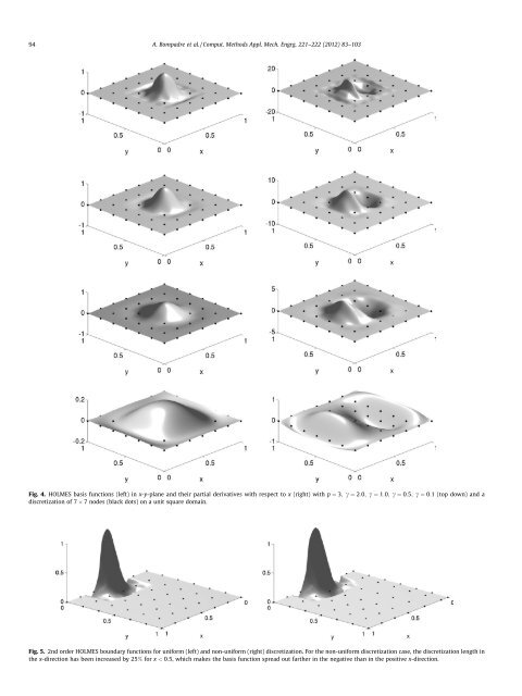
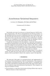
94 A. Bompadre et al. / Comput. Methods Appl. Mech. Engrg. 221–222 (2012) 83–103Fig. 4. HOLMES basis functions (left) in x-y-plane <strong>and</strong> their partial derivatives with respect to x (right) with p ¼ 3; c ¼ 2:0; c ¼ 1:0; c ¼ 0:5; c ¼ 0:1 (top down) <strong>and</strong> adiscretization <strong>of</strong> 7 7 nodes (black dots) on a unit square domain.Fig. 5. 2nd <strong>order</strong> HOLMES boundary functions for uniform (left) <strong>and</strong> non-uniform (right) discretization. For the non-uniform discretization case, the discretization length inthe x-direction has been increased by 25% for x < 0:5, which makes the basis function spread out farther in the negative than in the positive x-direction.
A. Bompadre et al. / Comput. Methods Appl. Mech. Engrg. 221–222 (2012) 83–103 95B-splines are used as window functions. All examples presented inthis section make use <strong>of</strong> a uniform discretization with characteristicdiscretization length h along each coordinate axis, <strong>and</strong> Gaussquadrature subordinate to an auxiliary triangulation is used fornumerical integration. In the case <strong>of</strong> B-splines, both the nodes inthe physical space <strong>and</strong> the knots in the parameter space are uniformlydistributed. Numerical quadrature is performed in d dimensionsfor FEM basis functions with n d GPGauss points per finiteelement. For B-splines Gauss integration with n d GPGauss points isperformed in the parameter space on the intervals between adjacentknots <strong>and</strong> for HOLMES <strong>and</strong> MLS functions with n d GPGausspoints on the intervals between adjacent nodes in the physicalspace. Boundary conditions on derivatives are imposed by means<strong>of</strong> Lagrange multipliers, as pointed out in Section 5.2.2 <strong>of</strong> [9], whereverB-splines were used. For HOLMES <strong>and</strong> MLS functions, Lagrangemultipliers are used to impose boundary conditions bothon function values <strong>and</strong> derivatives following the collocation pointmethod as described in Subsection 3.3.2, Chapter 10 <strong>of</strong> [14].According to the collocation point method, the interpolation functionsfor Lagrange multipliers are Dirac-delta functions centered ata set <strong>of</strong> collocation points where the boundary conditions are imposedexactly. In all our examples, the collocation points correspondto the discretization nodes on the Dirichlet boundary <strong>of</strong>the domain.Before applying HOLMES to solve PDE’s, in the following numericalexamples we assess the ability <strong>of</strong> HOLMES to reproduce asmooth function, <strong>and</strong> to pass a ‘‘patch test’’ in the spirit <strong>of</strong> Example5.1 <strong>of</strong> [2]. We test HOLMES to reproduce the functions uðxÞ ¼sinðxÞin the interval ½0; 2pŠ, <strong>and</strong> uðxÞ ¼expðxÞ in the interval ½0; 1Š usingp ¼ 3 <strong>and</strong> c ¼ 0:3 orc ¼ 0:8. As shown in Fig. 6 <strong>and</strong> in Table 2, theL 2 ; H 1 , <strong>and</strong> H 2 error seminorms converge at a rate equal to, or higherthan, the theoretical rate <strong>of</strong> convergence given by Theorem 3, forboth functions <strong>and</strong> values <strong>of</strong> c. For the patch test, we consider thedisplacement uðxÞ <strong>of</strong> an elastic beam in the interval ½0; 1Š, subjectedto the boundary conditions uð0Þ ¼uð1Þ ¼0; u 0 ð0Þ ¼1, <strong>and</strong>u 0 ð1Þ ¼ 1, so that the deformed configuration is represented by aquadratic polynomial. Second-<strong>order</strong> HOLMES can reproduce exactlyquadratic functions <strong>and</strong>, as discussed in [2], the patch-test isintended to assess the consistency <strong>of</strong> HOLMES <strong>and</strong> the accuracy <strong>of</strong>the numerical quadrature used. We use seven nodes to discretizethe domain [0,1], using both uniform <strong>and</strong> non uniform nodal spacing.The patch test is performed using p ¼ 3 <strong>and</strong> c ¼ 0:3. Table 3tabulates the error seminorms with respect to the exact solutionfor different numbers <strong>of</strong> quadrature points between adjacent nodes.When a uniform nodal distribution is used, the exact solution isrecovered within machine precision with 32 quadrature points.Table 2Convergence rates for HOLMES <strong>approximation</strong> to sinðxÞ in the interval ½0; 2pŠ, <strong>and</strong> toexpðxÞ in the interval ½0; 1Š, for c ¼ 0:3 <strong>and</strong> c ¼ 0:8.uðxÞ Domain c L 2 H 1 H 2sinðxÞ ½0; 2pŠ 0.3 3.46 2.23 1.030.8 3.39 2.13 1.03expðxÞ ½0; 1Š 0.3 3.45 2.18 1.020.8 3.37 2.09 1.02For the non-uniform nodal distribution test, the convergence towardthe exact solution is slower <strong>and</strong> requires more quadraturepoints, as already observed in [2].In all subsequent examples, the number <strong>of</strong> quadrature points ischosen so as to ensure accuracy in the evaluation <strong>of</strong> HOLMES.7.1. Elastic rod under sine loadThe static displacements uðxÞ <strong>of</strong> a linearly elastic rod with unitmaterial <strong>and</strong> geometry parameters <strong>and</strong> fixed ends under sine loadare governed by the partial differential equationu xx ðxÞ ¼sinð2pxÞ;x 2½0; 1Š; uð0Þ ¼uð1Þ ¼0:ð82ÞApproximate solutions to (82) can be obtained by a Bubnov–Galerkin method using different types <strong>of</strong> basis functions. In Fig. 7we compare the convergence resulting from second-<strong>order</strong> HOLMES,B-spline, MLS <strong>and</strong> FEM, respectively. To this end, we use HOLMES<strong>and</strong> MLS shape functions with the same range r 3;HOLMES ¼r MLS ¼ 3h. The HOLMES shape functions are constructed <strong>and</strong> evaluatedwith p ¼ 3; c ¼ 0:8, <strong>and</strong> a numerical tolerance ¼ 1e 10with respect to (81). HOLMES is expected to attain optimal rates<strong>of</strong> convergence for both the L 2 - <strong>and</strong> H 1 -error norms. The accuracy<strong>of</strong> B-splines, MLS functions, <strong>and</strong> HOLMES is comparable <strong>and</strong> markedlybetter than the one achieved by finite element basis functions.We choose n GP ¼ 2 for the FEM <strong>and</strong> B-spline basis functions, <strong>and</strong>n GP ¼ 6 for the HOLMES <strong>and</strong> MLS functions, respectively. Thus,HOLMES <strong>and</strong> MLS require a slightly larger range <strong>and</strong> more integrationpoints than B-splines for a comparable performance. However,in contrast to B-splines, HOLMES <strong>and</strong> MLS can be applied withunstructured nodal sets, which greatly increases their range <strong>of</strong>applicability. We mention in passing that the computational cost<strong>of</strong> the evaluation <strong>of</strong> HOLMES <strong>and</strong> MLS basis functions in our MATLABimplementation is similar. Figs. 8 <strong>and</strong> 9 show how the accuracyobtained from HOLMES depends on c <strong>and</strong> p. In all cases, optimalconvergence is achieved for p P 3, as expected from the analysis10 −210 −2Error seminorms10 0 h10 −410 −610 −810 −2 10 −1L 2 η = 3.46H 1 η = 2.23H 2 η = 1.03Error seminorms10 −410 −610 −810 −1010 0 hL 2 η = 3.45H 1 η = 2.18H 2 η = 1.0210 −2 10 −1Fig. 6. Convergence <strong>of</strong> the L 2 ; H 1 , <strong>and</strong> H 2 error seminorms with respect to uniform nodal spacing h for HOLMES <strong>approximation</strong> to sinðxÞ in the interval ½0; 2pŠ (left), <strong>and</strong> toexpðxÞ in the interval ½0; 1Š (right) for c ¼ 0:3. The rates <strong>of</strong> convergence g for the error seminorms are reported in each plot.