Digital Signal Processing Chapter 7: Parametric Spectrum Estimation

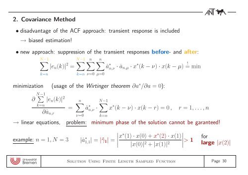
2. Covariance Method• disadvantage of the ACF approach: transient response is included→ biased estimation!• new approach: suppression of the transient responses before- and after:N−1∑N−1∑ n∑ n∑|e n (k)| 2 = â ∗ n,ν · â n,µ · x ∗ (k − ν) · x(k − µ) = ! mink=nk=nν=0µ=0minimization (usage of the Wirtinger theorem ∂a ∗ /∂a = 0):∂ N−1 ∑k=n|e n (k)| 2∂â n,r=→ linear equations,n∑â ∗ n,ν ·ν=0N−1∑k=nexample: n = 1, N = 3 |â ∗ 1,1| = |ˆγ 1 | =x ∗ (k − ν) · x(k − r) = 0 ,r = 1, ...,nproblem: minimum phase of the solution cannot be garanteed!∣ x ∗ (1) · x(0) + x ∗ (2) · x(1) ∣∣∣∣> 1|x(0)| 2 + |x(1)| 2forlarge |x(2)|Solution Using Finite Length Sampled Function Page 30