Cosmological Perturbation Theory, 26.4.2011 version

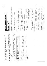
6 PERTURBATIONS IN FOURIER SPACE 14andso that the vector part of δg µν isFor the tensor part,⎡Eij V = −i2k (k iE j + k j E i ) = − i ⎣2⎡δgµν V = a 2 ⎢⎣−B 1 −B 2⎤−B 1 −iE 1−B 2 −iE 2⎤E 1E 2⎦ , (6.14)E 1 E 2⎥⎦ . (6.15)δ ik k k E T ij ≡ ∑ ik i E T ij = 0 ⇒ ET 3j ≡ ET j3 = 0 (6.16)so that⎡Eij T = ⎣E11 T E12TE12 T −E11T⎤⎦ . (6.17)The tensor part of δg µν becomes⎡δgµν T = a2 ⎢⎣2E11 T 2E12T2E12 T −2E11T⎤ ⎡⎥⎦ = a2 ⎢⎣⎤h + h ×⎥h × −h +⎦ , (6.18)where we have denoted the two gravitational wave polarization amplitudes by E T 11 = 1 2 h + andE T 12 = 1 2 h ×.We see how the scalar part of the perturbation is associated with the time direction, thewave direction ⃗ k and the trace. The vector part is associated with the two remaining spacedirections, those transverse to the wave vector. Thus the vectors have only two independentcomponents. The tensor part is also associated with these two transverse directions; being alsosymmetric and traceless, it thus has only two independent components.Putting all together, the full metric perturbation (for a Fourier mode in the z direction) is⎡δg µν = a 2 ⎢⎣⎤−2A −B 1 −B 2 +iB−B 1 2(−D + 1 3 E) + h + h × −iE 1−B 2 h × 2(−D + 1 3 E) − h + −iE 2+iB −iE 1 −iE 2 2(−D − 2 3 E)6.1 Gauge Transformation in Fourier Space⎥⎦ . (6.19)Consider then how the gauge transformation appears in Fourier space. We need now the Fouriertransform of the gauge transformation vectorξ µ (η,⃗x) = ∑ ⃗ kξ µ ⃗ k(η)e i⃗ k·⃗x . (6.20)