Cosmological Perturbation Theory, 26.4.2011 version
Cosmological Perturbation Theory, 26.4.2011 version
Cosmological Perturbation Theory, 26.4.2011 version

You also want an ePaper? Increase the reach of your titles
YUMPU automatically turns print PDFs into web optimized ePapers that Google loves.
10 FIELD EQUATIONS FOR SCALAR PERTURBATIONS IN THE NEWTONIAN GAUGE23Separating the δG i j equation into its trace and traceless part (the trace of δi jof (Ψ − Φ) ,ij is ∇ 2 (Ψ − Φ)) the full set of Einstein equations isis 3, and the trace3H(Ψ ′ + HΦ) − ∇ 2 Ψ = −4πGa 2 δρ N (10.3)(Ψ ′ + HΦ) ,i = 4πGa 2 (¯ρ + ¯p)v N ,i (10.4)Ψ ′′ + H(Φ ′ + 2Ψ ′ ) + (2H ′ + H 2 )Φ + 1 3 ∇2 (Φ − Ψ) = 4πGa 2 δp N (10.5)The off-diagonal part of the last equation givesIn Fourier space this reads(∂ i ∂ j − 1 3 δi j ∇2 )(Ψ − Φ) = 8πGa 2¯p(∂ i ∂ j − 1 3 δi j ∇2 )Π. (10.6)(Ψ − Φ) ,ij = 8πGa 2¯pΠ ,ij for i ≠ j . (10.7)−k i k j (Ψ ⃗k − Φ ⃗k ) = − k ik jk 2 8πGa2¯pΠ ⃗k for i ≠ j . (10.8)(with the Liddle&Lyth Fourier convention for Π). Since we can always rotate the backgroundcoordinate system so that more than one of the components of ⃗ k are non-zero, this means thatk 2 (Ψ ⃗k − Φ ⃗k ) = 8πGa 2¯pΠ ⃗k for ⃗ k ≠ ⃗0 . (10.9)The 0 th Fourier component represents a constant offset. But the split into a background and aperturbation is always chosen so that the spatial average of the perturbation vanishes (and thebackground value thus represents the spatial average of the full perturbed quantity).Thus we have (going back to ⃗x-space)Ψ − Φ = 8πGa 2¯pΠ. (10.10)Likewise, since the spatial average of a perturbation is always zero, the equality of gradientsof two perturbations means the equality of those perturbations themselves. Thus Eq. (10.4) saysthatΨ ′ + HΦ = 4πGa 2 (¯ρ + ¯p)v N = 3 2 H2 (1 + w)v N . (10.11)Inserting this into Eq. (10.3) gives∇ 2 Ψ = 4πGa 2¯ρ [ δ N + 3H(1 + w)v N] , (10.12)where we have defined the relative energy density perturbationδ ≡δρ¯ρ. (10.13)(and w ≡ ¯p/¯ρ).The final form of the Einstein equations can be divided into two constraint equations∇ 2 Ψ = 4πGa 2¯ρ [ δ N + 3H(1 + w)v N] (10.14)Ψ − Φ = 8πGa 2¯pΠ (10.15)that apply to any given time slice, and to two evolution equationsΨ ′ + HΦ = 3 2 H2 (1 + w)v N (10.16)Ψ ′′ + H(Φ ′ + 2Ψ ′ ) + (2H ′ + H 2 )Φ + 1 3 ∇2 (Φ − Ψ) = 4πGa 2 δp N . (10.17)