Preprint

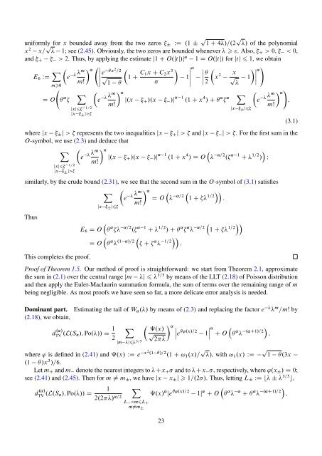
uniformly for x bounded away from the two zeros ˙ WD .1 ˙ p1C 4/=.2 p / of the polynomialx 2 x= p 1; see (2.45). Obviously, the two zeros are bounded whenever ". Also, C > 0, < 0,and C > 2. Thus, by applying the estimate j1 C O.jtj/j˛ 1 D O.jtj/ for jtj 1, we obtainE 6 WD X ˛e me x2 =2p 1 C C 1x C C 2 x 31ˇm! ˇm01 ˇ˛ ˇˇˇˇ x 2 x˛!p21ˇˇˇˇD O ˛X˛ e mX˛!j.x C /.x /j˛ 1 .1 C x 4 / C e ˛˛ m;m!m!jxj 1=2jx ˙j>where jx ˙j > represents the two inequalities jx C j > and jx j > . For the first sum in theO-symbol, we use (2.3) and deduce thatX˛e mj.x C /.x /j˛ 1 .1 C x 4 / D O ˛=2 .˛ 1 C 1=2 / Im!jxj 1=2jx ˙j>similarly, by the crude bound (2.31), we see that the second sum in the O-symbol of (3.1) satisfiesX˛e mD O1 ˛=2 C 1=2 :m!ThusThis completes the proof.jx˙jE 6 D O ˛ ˛=2 .˛ 1 C 1=2 / C ˛˛1 ˛=2 C 1=2D O ˛ .1 ˛/=2 C ˛ 1=2 :Proof of Theorem 1.5. Our method of proof is straightforward: we start from Theorem 2.1, approximatethe sum in (2.1) over the central range jm j 3=5 by means of the LLT (2.18) of Poisson distributionand then apply the Euler-Maclaurin summation formula, the sum of terms over the remaining range of mbeing negligible. As most proofs we have seen so far, a more delicate error analysis is needed.Dominant part.(2.18), we obtain,jx˙j(3.1)Estimating the tail of W˛./ by means of (2.3) and replacing the factor e m =m! byd .˛/TV .L.S n/; Po.// D 1 2jmX ‰.x/˛'.x/=2pˇˇˇej 2 3=5ˇ1ˇ˛ C O ˛ .˛C1/=2 ;where ' is defined in (2.41) and ‰.x/ WD e x2 .1 /=2 .1 C ! 1 .x/= p /, with ! 1 .x/ WD p 1 .3x.1 /x 3 /=6.Let m C and m denote the nearest integers to Cx C and to Cx , respectively, where '.x˙/ D 0;see (2.41) and (2.45). Then for m 6D m˙, we have jx x˙j 1=.2/. Thus, letting L˙ WD b ˙ 3=5 c,d .˛/TV .L.S n/; Po.// D12.2/˛=2XL