Preprint

More documents

Recommendations

Info

This says that Poisson approximation to binomial distribution is good as long as p is small. Observe thatwhen np ! 1 the O-term in (1.1) is asymptotically smaller than the dominant term, while in the caseof bounded np, the right-hand side becomes an upper bound. Thus (1.1) extends Poisson’s original limittheorem in two directions: in degree of precision and in range of variations of p. Such an extension hassince attracted the interest of many probabilists and many powerful tools have been developed; see, inparticular, [4, 5, 8, 9, 16, 21, 27] and the references therein for more information.Second-order refinement. A natural question regarding the approximation (1.1) is that how good theleading term is. Or, is the error term optimal? This raises the question of second-order expansion inPoisson approximation problems, which, as far as we were aware, was first addressed by Kerstan in [18].His results implicitly imply that if p D o.1/, then ( WD np)whered TV .Bi.nI p/; Po.// D pT C O.p 2 /; (1.2)T WD 1 4Xj0 jj !ˇˇˇˇ e .j / 2 jNote that T D .2e/ 1=2 .1 C ‚. 1 //; see also [9, 15]. In particular, for p D o.1/ and ! 1,d TV .Bi.nI p/; Po.// D p p 1 C O p C 1 I (1.3)2ecompare (1.1). The asymptotic nature of Prokhorov’s result (1.1) is now clearer. Note that the minimumerror (of the O-term) is reached when p D 1 , or when p D n 1=2 . Kerstan’s result was later extendedin [2, 4, 8, 11, 27] by different approaches; see also the book [5] for more details.New uniform approximations.distanceˇ :Instead of the total variation distance, we consider in this paper thed .˛/TV .L.X /; L.Y // WD 1 2XjP.X D m/ P.Y D m/j˛ ; (1.4)mbetween the distributions of the two discrete random variables X and Y , where, here and throughout thispaper, ˛ > 0 is a fixed constant. The interest of considering d .˛/TV is multifold. First, such a quantityis, modulo power, the natural analogue of the usual `p-norm; see [25, Ch. 2] and [27]. When ˛ D 1the above quantity coincides with the usual total variation distance d TV . Second, it can be regarded as aneffective measure of robustness of Poisson approximation; see Corollary 1.4 and its discussions. Third,several approaches to Poisson approximation apply well only for special values of ˛ but not for all. Thus,its consideration also introduces more methodological interests. Indeed, most of our proofs will largelysimplify if we consider only the case when ˛ 1.Throughout this paper, q WD 1 p.Theorem 1.1. If p 1=2 and WD np ! 1, thend .˛/.1TV .Bi.nI p/; Po.// D p˛ ˛/=2J˛.p/where J˛.p/ is bounded for p 2 .0; 1/ and ˛ > 0, and defined by1J˛.p/ De ˛t 2 =2e pt 2 =.2q/p 12.2/˛=2 p˛ˇ q ˇZ 111 C O .˛C1/=2 C 1 ; (1.5)˛dt: (1.6)2
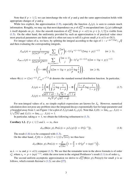
Note that if p > 1=2, we can interchange the role of p and q and the same approximation holds withappropriate changes of p and q.While less explicit, the approximation (1.9), especially the function J˛.p/, is seen to contain muchinformation. Roughly, we may say that most dependence on p of d .˛/TV is encapsulated into J˛.p/ (although itself depends on p). Also the smooth transition of d .˛/TV from p D o.1/ to p 2 Œ"; 1=2 is visible from(1.5). On the other hand, the uniformity provided by such an approximation is of practical value sincemost practical parameters are finite and it is often not easy to tell if a given small p is o.1/ or O.1/.For integer values of ˛, we have, by splitting the integral according to the sign of 1 e px2 =.2q/ = p qand then evaluating the corresponding integrals,J 2m .p/ DJ 2mC1 .p/ D1 X2.2/ m 1=2 p 2m12.2/ m p 2mC1 3 4ˆ0j2mX0j2mC1s 2mj 2m C 1. 1/ j q .j 1/=2 .2mq C pj / 1=2 .m 1/;j..2m C 1/q C pj / 1 p log 1 q. 1/ j q .j 1/=2 ..2m C 1/q C pj / 1=2!!; .m 0/;where ˆ.x/ WD .2/ 1=2 R x1 e t 2 =2 dt denotes the standard normal distribution function. In particular,s! s!!J 1 .p/ D 2 p ˆ 1p log 11 pˆ1 pp log 1; (1.7)1 pp p pq.1 C q/ 2 2q C 1 C qJ 2 .p/ D4 p p 2p :q.1 C q/For non-integral values of ˛, no simple explicit expressions are known for J˛. However, numericalcalculation does not pose any problem since the integrand decays exponentially fast for large parameter andp bounded away from 1; see Figure 1 for a plot of J 1 .p/ and J 1=2 .p/. Note that J 1 .0/ WD lim t!0 C J 1 .t/ D1= p 2e and J 1 .1/ WD lim t!1 J 1 .t/ D 1.In particular, taking ˛ D 1, we obtain the following refinement to (1.3).Corollary 1.2. If p 1=2 and ! 1, thend TV .Bi.nI p/; Po.// D pJ 1 .p/ 1 C O 1 : (1.8)The result (1.8) is to be compared with (1.3).On the other hand, J 0 1 .0/ D J 1.0/=2 D 1=.2 p 2e/; we thus haved TV .Bi.nI p/; Po.// Dp p2e1 C p 2 C O p2 C .np/ 1 ;as ! 1 and p D o.1/; compare (1.3). We see that the remainder term in the above formula is of orderrn 2, where r n D p C .np/ 1=2 , while the error term in the original Prokhorov’s result (1.1) is of order r n .The second uniform asymptotic approximation we derive to d .˛/TV .Bi.nI p/; Po.np// for small p is asfollows, which extends Kerstan’s (1.2); see also [27].3
Page 1: Uniform asymptotics of Poisson appr
Page 5 and 6: On the other hand, another natural
Page 7 and 8: To prove Theorem 2.1, let ı n;m WD
Page 9 and 10: Proof. The upper bound of (2.7) fol
Page 11 and 12: 2.5 The usual LLT for S nWith the a
Page 13 and 14: It follows thatE.t/ C 22 .eit 1/ 2
Page 15 and 16: Proposition 2.10. Assume K > 0 an
Page 17 and 18: Note that by (2.35) the terms insid
Page 19 and 20: for sufficiently small , where c 4
Page 21 and 22: we can apply the same proof used fo
Page 23: uniformly for x bounded away from t
Page 26 and 27: andmlog 1 D log.1nSubstituting thes
Page 28: [24] YU. V. PROKHOROV, Asymptotic b

Preprint

Create successful ePaper yourself

Delete template?

Save as template?