- Page 2:
Ocean Modelling for Beginners
- Page 6:
Assoc. Prof. Jochen KämpfSchool of
- Page 10:
viPrefaceAccess to a standard compu
- Page 16:
Contentsix3.7.3 Apparent Forces . .
- Page 20:
Contentsxi4.2.3 The Shallow-Water M
- Page 24:
Contentsxiii5.9 Exercise 13: Inclus
- Page 28:
Contentsxv6.13.3 Results...........
- Page 32:
2 1 RequirementsMicrosoft Windows O
- Page 36:
Chapter 2MotivationAbstract This ch
- Page 40:
2.1 The Decay Problem 7Fig. 2.1 Evo
- Page 44:
2.2 First Steps with Finite Differe
- Page 48:
2.2 First Steps with Finite Differe
- Page 52:
2.3 Exercise 1: The Decay Problem 1
- Page 56:
2.4 Detection and Elimination of Er
- Page 60:
Chapter 3Basics of Geophysical Flui
- Page 64:
3.3 Location and Velocity 19Fig. 3.
- Page 68:
3.5 Visualisation of a Wave Using S
- Page 72: 3.5 Visualisation of a Wave Using S
- Page 76: 3.6 Exercise 2: Wave Interference 2
- Page 80: 3.7 Forces 273.7 Forces3.7.1 What F
- Page 84: 3.7 Forces 293.7.6 Interpretation o
- Page 88: 3.8 Fundamental Conservation Princi
- Page 92: 3.8 Fundamental Conservation Princi
- Page 96: 3.9 Gravity and the Buoyancy Force
- Page 100: 3.10 Exercise 3: Oscillations of a
- Page 104: 3.10 Exercise 3: Oscillations of a
- Page 108: 3.11 The Pressure-Gradient Force 41
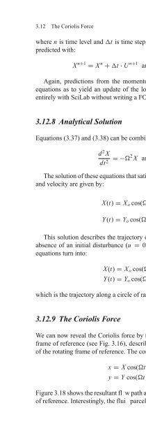
- Page 112: 3.12 The Coriolis Force 43where red
- Page 116: 3.12 The Coriolis Force 45operates
- Page 120: 3.12 The Coriolis Force 47where the
- Page 126: 50 3 Basics of Geophysical Fluid Dy
- Page 130: 52 3 Basics of Geophysical Fluid Dy
- Page 134: 54 3 Basics of Geophysical Fluid Dy
- Page 138: 56 3 Basics of Geophysical Fluid Dy
- Page 142: 58 3 Basics of Geophysical Fluid Dy
- Page 146: 60 3 Basics of Geophysical Fluid Dy
- Page 150: 62 3 Basics of Geophysical Fluid Dy
- Page 154: Chapter 4Long Waves in a ChannelAbs
- Page 158: 4.1 More on Finite Differences 67
- Page 162: 4.2 Long Surface Gravity Waves 69Fi
- Page 166: 4.2 Long Surface Gravity Waves 71Fi
- Page 170: 4.2 Long Surface Gravity Waves 734.
- Page 174:
4.2 Long Surface Gravity Waves 75EN
- Page 178:
4.4 Exercise 6: The Flooding Algori
- Page 182:
4.4 Exercise 6: The Flooding Algori
- Page 186:
4.4 Exercise 6: The Flooding Algori
- Page 190:
4.5 The Multi-Layer Shallow-Water M
- Page 194:
4.6 Exercise 7: Long Waves in a Lay
- Page 198:
4.6 Exercise 7: Long Waves in a Lay
- Page 202:
4.6 Exercise 7: Long Waves in a Lay
- Page 206:
92 5 2D Shallow-Water ModellingFig.
- Page 210:
94 5 2D Shallow-Water Modelling5.1.
- Page 214:
96 5 2D Shallow-Water Modellinggrav
- Page 218:
98 5 2D Shallow-Water Modellingwher
- Page 222:
100 5 2D Shallow-Water Modellingv n
- Page 226:
102 5 2D Shallow-Water ModellingFig
- Page 230:
104 5 2D Shallow-Water Modelling5.5
- Page 234:
106 5 2D Shallow-Water Modelling•
- Page 238:
108 5 2D Shallow-Water ModellingFig
- Page 242:
110 5 2D Shallow-Water ModellingFig
- Page 246:
112 5 2D Shallow-Water Modelling5.9
- Page 250:
114 5 2D Shallow-Water Modellingwhe
- Page 254:
116 5 2D Shallow-Water Modellingzer
- Page 258:
118 5 2D Shallow-Water ModellingFig
- Page 262:
120 6 Rotational EffectsStep 1: Pre
- Page 266:
122 6 Rotational Effectsdiffusion a
- Page 270:
124 6 Rotational Effectsis called t
- Page 274:
126 6 Rotational Effectsd(PV)dtwher
- Page 278:
128 6 Rotational Effectswhere T is
- Page 282:
130 6 Rotational EffectsFig. 6.4 Ba
- Page 286:
132 6 Rotational Effectsappearance
- Page 290:
134 6 Rotational Effects6.6.2 Insta
- Page 294:
136 6 Rotational EffectsFig. 6.9 Ex
- Page 298:
138 6 Rotational Effectswhere Q x a
- Page 302:
140 6 Rotational EffectsFig. 6.12 S
- Page 306:
142 6 Rotational EffectsFig. 6.13 S
- Page 310:
144 6 Rotational EffectsFig. 6.14 S
- Page 314:
146 6 Rotational Effectsand uniform
- Page 318:
148 6 Rotational Effects6.10 Exerci
- Page 322:
150 6 Rotational Effectsassumption,
- Page 326:
152 6 Rotational EffectsFig. 6.20 I
- Page 330:
154 6 Rotational EffectsThe solutio
- Page 334:
156 6 Rotational Effectsand a radiu
- Page 338:
158 6 Rotational Effectsfirs analyt
- Page 342:
160 6 Rotational EffectsFig. 6.26 E
- Page 346:
162 6 Rotational Effects6.15.5 Addi
- Page 350:
164 6 Rotational EffectsFig. 6.30 B
- Page 354:
166 6 Rotational EffectsFig. 6.32 S
- Page 358:
BibliographyArakawa, A., and Lamb,
- Page 362:
List of Exercises• Exercise 1: Th
- Page 366:
174 IndexFFinite differencesexplici