- Page 2:
Ocean Modelling for Beginners
- Page 6:
Assoc. Prof. Jochen KämpfSchool of
- Page 10:
viPrefaceAccess to a standard compu
- Page 16:
Contentsix3.7.3 Apparent Forces . .
- Page 20:
Contentsxi4.2.3 The Shallow-Water M
- Page 24:
Contentsxiii5.9 Exercise 13: Inclus
- Page 28:
Contentsxv6.13.3 Results...........
- Page 32:
2 1 RequirementsMicrosoft Windows O
- Page 36:
Chapter 2MotivationAbstract This ch
- Page 40:
2.1 The Decay Problem 7Fig. 2.1 Evo
- Page 44:
2.2 First Steps with Finite Differe
- Page 48:
2.2 First Steps with Finite Differe
- Page 52:
2.3 Exercise 1: The Decay Problem 1
- Page 56:
2.4 Detection and Elimination of Er
- Page 60:
Chapter 3Basics of Geophysical Flui
- Page 64:
3.3 Location and Velocity 19Fig. 3.
- Page 68:
3.5 Visualisation of a Wave Using S
- Page 72:
3.5 Visualisation of a Wave Using S
- Page 76:
3.6 Exercise 2: Wave Interference 2
- Page 80:
3.7 Forces 273.7 Forces3.7.1 What F
- Page 84:
3.7 Forces 293.7.6 Interpretation o
- Page 88:
3.8 Fundamental Conservation Princi
- Page 92:
3.8 Fundamental Conservation Princi
- Page 96:
3.9 Gravity and the Buoyancy Force
- Page 100:
3.10 Exercise 3: Oscillations of a
- Page 104:
3.10 Exercise 3: Oscillations of a
- Page 108:
3.11 The Pressure-Gradient Force 41
- Page 112:
3.12 The Coriolis Force 43where red
- Page 116:
3.12 The Coriolis Force 45operates
- Page 120:
3.12 The Coriolis Force 47where the
- Page 124:
3.12 The Coriolis Force 49where n i
- Page 128:
3.13 The Coriolis Force on Earth 51
- Page 132:
3.14 Exercise 4: The Coriolis Force
- Page 136:
3.14 Exercise 4: The Coriolis Force
- Page 140:
3.15 Turbulence 57(10 cm/s, 0 cm/s)
- Page 144:
3.15 Turbulence 593.15.5 Turbulence
- Page 148:
3.17 Scaling 613.16.2 Boundary Cond
- Page 152:
3.17 Scaling 63where T i is the ine
- Page 156:
66 4 Long Waves in a ChannelOn the
- Page 160:
68 4 Long Waves in a ChannelThe tru
- Page 164:
70 4 Long Waves in a ChannelIt can
- Page 168:
72 4 Long Waves in a ChannelFig. 4.
- Page 172:
74 4 Long Waves in a ChannelZero-gr
- Page 176:
76 4 Long Waves in a ChannelFig. 4.
- Page 180:
78 4 Long Waves in a ChannelFig. 4.
- Page 184:
80 4 Long Waves in a Channel3. True
- Page 188:
82 4 Long Waves in a Channelplace w
- Page 192:
84 4 Long Waves in a Channelwhere h
- Page 196:
86 4 Long Waves in a ChannelFig. 4.
- Page 200:
88 4 Long Waves in a Channel4.6.8 C
- Page 204:
Chapter 52D Shallow-Water Modelling
- Page 208:
5.1 Long Waves in a Shallow Lake 93
- Page 212:
5.3 Exercise9:WaveRefraction 95Fig.
- Page 216:
5.3 Exercise9:WaveRefraction 97Fig.
- Page 220:
5.4 The Wind-Forced Shallow-Water M
- Page 224:
5.5 Exercise 10: Wind-Driven Flow i
- Page 228:
5.5 Exercise 10: Wind-Driven Flow i
- Page 232: 5.6 Movement of Tracers 105In all s
- Page 236: 5.7 Exercise 11: Eulerian Advection
- Page 240: 5.8 Exercise 12: Trajectories 1095.
- Page 244: 5.9 Exercise 13: Inclusion of Nonli
- Page 248: 5.10 Exercise 14: Island Wakes 1135
- Page 252: 5.10 Exercise 14: Island Wakes 1155
- Page 256: 5.10 Exercise 14: Island Wakes 1175
- Page 260: Chapter 6Rotational EffectsAbstract
- Page 264: 6.3 Exercise 15: Coastal Kelvin Wav
- Page 268: 6.4 Geostrophic Flow 123Sect. 3.17)
- Page 272: 6.4 Geostrophic Flow 125Fig. 6.2 Ex
- Page 276: 6.4 Geostrophic Flow 127In a multi-
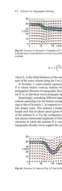
- Page 280: 6.5 Exercise 16: Topographic Steeri
- Page 286: 132 6 Rotational Effectsappearance
- Page 290: 134 6 Rotational Effects6.6.2 Insta
- Page 294: 136 6 Rotational EffectsFig. 6.9 Ex
- Page 298: 138 6 Rotational Effectswhere Q x a
- Page 302: 140 6 Rotational EffectsFig. 6.12 S
- Page 306: 142 6 Rotational EffectsFig. 6.13 S
- Page 310: 144 6 Rotational EffectsFig. 6.14 S
- Page 314: 146 6 Rotational Effectsand uniform
- Page 318: 148 6 Rotational Effects6.10 Exerci
- Page 322: 150 6 Rotational Effectsassumption,
- Page 326: 152 6 Rotational EffectsFig. 6.20 I
- Page 330: 154 6 Rotational EffectsThe solutio
- Page 334:
156 6 Rotational Effectsand a radiu
- Page 338:
158 6 Rotational Effectsfirs analyt
- Page 342:
160 6 Rotational EffectsFig. 6.26 E
- Page 346:
162 6 Rotational Effects6.15.5 Addi
- Page 350:
164 6 Rotational EffectsFig. 6.30 B
- Page 354:
166 6 Rotational EffectsFig. 6.32 S
- Page 358:
BibliographyArakawa, A., and Lamb,
- Page 362:
List of Exercises• Exercise 1: Th
- Page 366:
174 IndexFFinite differencesexplici