Representations of Lie algebras, Casimir operators and their ...

More documents

Recommendations

Info

where the potentially half–integer valued parameter p is traditionallyreplaced by the integer n = 2p+1 > 0. Once we have established thatE is determined by the value of p by equation (22) we also see thatH E coincides with the representation space of the so(4) irreduciblerepresentation labelled by p and q = p. On H E we may also writeequation (21) in the form( MQ2C 1 + C 2 = −4 2Ĥ + 1 )(23)2since both C 1 + C 2 and Ĥ take a constant value on H E. While itmay be tempting to consider this to be an operator identity validon the whole Hilbert space H, we don’t consider such interpretationlegitimate. In particular, on scattering states (E > 0) we even havea different Lie algebra. Therefore, equation (23) should be consideredat most on the bound state sector of our Hilbert space H.To sum up, we have seen that the spectrum of hydrogen atom canbe derived using the theory of Lie algebras, without explicit constructionof eigenfunctions. More precisely, we have derived a necessarycondition (22) that any energy eigenvalue must satisfy. That this formulais physically relevant for all values of p ≥ 0 such that 2p ∈ Zis not a consequence of the computation just shown and shall be establishedby other means (e.g. by an explicit construction of s–statesintroduced above). Once the existence of at least one state with theenergy E n = − MQ2 1is shown, the degeneracy n 2 of the energy level2 2 n 2E n also follows directly from algebraic considerations.3 Generalized Casimir invariantsAs was shown by Kirillov in [8] and will be explained below, Casimiroperators are in one–to–one correspondence with polynomial invariantscharacterizing orbits of the coadjoint representation of g. Thesearch for invariants of the coadjoint representation is algorithmicand amounts to solving a system of linear first order partial differentialequations [9, 10, 11, 12, 13, 14, 15, 16, 17]. Alternatively, globalproperties of the coadjoint representation can be used [13, 18, 19, 20].In general, solutions are not necessarily polynomials and we shall callthe nonpolynomial solutions generalized Casimir invariants.For certain classes of Lie algebras, including semisimple Lie algebras,perfect Lie algebras, nilpotent Lie algebras, and more generallyalgebraic Lie algebras, all invariants of the coadjoint representationare functions of polynomial ones [9, 10].On the other hand, in the representation theory of solvable Liealgebras their invariants are not necessarily polynomials, i.e. they can12
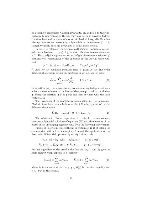
e genuinely generalized Casimir invariants. In addition to their importancein representation theory, they may occur in physics. Indeed,Hamiltonians and integrals of motion of classical integrable Hamiltoniansystems are not necessarily polynomials in the momenta [21, 22],though typically they are invariants of some group action.In order to calculate the (generalized) Casimir invariants we considersome basis (e 1 , . . . , e n ) of g, in which the structure constants arec ij k . The coadjoint representation ad ∗ of g is the representation on g ∗obtained via transposition of the operators in the adjoint representation〈ad ∗ (x)φ, y〉 = −〈φ, ad(x)y〉, ∀x, y ∈ g, φ ∈ g ∗ .A basis for the coadjoint representation is given by the first orderdifferential operators acting on functions on g ∗ , i.e. vector fields,Ê k =n∑a,b=1be b c ∂ka , 1 ≤ k ≤ n. (24)∂e aIn equation (24) the quantities e a are commuting independent variables– the coordinates in the basis of the space g ∗ , dual to the algebrag. Using the relation (g ∗ ) ∗ ≃ g one can identify them with the basisvectors of g.The invariants of the coadjoint representation, i.e. the generalizedCasimir invariants, are solutions of the following system of partialdifferential equationsÊ k I(e 1 , . . . , e n ) = 0, k = 1, . . . , n. (25)The relation to Casimir operators, i.e. the 1–1 correspondencebetween polynomial solutions of equation (25) and the elements of thecenter of the enveloping algebra comes from the following observations.Firstly, it is obvious that both the operation on U(g) of taking thecommutator with a fixed element e k ∈ g and the application of thefirst order differential operator Êk satisfy Leibniz rule[e k , a 1 a 2 ] = [e k , a 1 ]a 2 + a 1 [e k , a 2 ], a 1 , a 2 ∈ U(g),Ê k (F 1 F 2 ) = Êk(F 1 )F 2 + F 1 Ê k (F 2 ), F 1 , F 2 ∈ C ∞ (g ∗ ).Further ingredient of the proof is the fact that [e k , ·] and Êk give thesame answer when applied to e l , namely[e k , e l ] =n∑c m kl e m , Ê k (e l ) =m=1n∑c m kl e m , (26)m=1where it is understood that e l ∈ g ⊂ U(g) in the first equality ande l ∈ (g ∗ ) ∗ in the second.13
Page 1 and 2: Representations of Lie algebras, Ca
Page 3 and 4: A representation ρ of g on V is fu
Page 5 and 6: mod J . We shall occasionally suppr
Page 7 and 8: i.e. it coincides up to a numerical
Page 9 and 10: (chosen dimensionless for convenien
Page 11: When we expand the expressions for
Page 15 and 16: References[1] E. E. Levi, “Sulla

Representations of Lie algebras, Casimir operators and their ...

You also want an ePaper? Increase the reach of your titles

Delete template?

Save as template?