Product distribution theory for control of multi-agent systems

Product distribution theory for control of multi-agent systemsChiu Fan LeePhysics Department, Oxford UniversityParks Road, Oxford OX1 3PU, U.K.c.lee1@physics.ox.ac.ukDavid H. WolpertMS 269-1, NASA Ames Research CenterMoffett Field, CA 94035, USAdhw@ptolemy.arc.nasa.govAbstractProduct Distribution (PD) theory is a new framework forcontrolling Multi-Agent Systems (MAS’s). First we reviewone motivation of PD theory, as the information-theoreticextension of conventional full-rationality game theory to thecase of bounded rational agents. In this extension the equilibriumof the game is the optimizer of a Lagrangian of the(probability distribution of) the joint state of the agents. Accordinglywe can consider a team game in which the sharedutility is a performance measure of the behavior of the MAS.For such a scenario the game is at equilibrium — the Lagrangianis optimized — when the joint distribution of theagents optimizes the system’s expected performance. Onecommon way to find that equilibrium is to have each agentrun a reinforcement learning algorithm. Here we investigatethe alternative of exploiting PD theory to run gradientdescent on the Lagrangian. We present computer experimentsvalidating some of the predictions of PD theory forhow best to do that gradient descent. We also demonstratehow PD theory can improve performance even when we arenot allowed to rerun the MAS from different initial conditions,a requirement implicit in some previous work.1. IntroductionProduct Distribution (PD) theory is a recently introducedbroad framework for analyzing, controlling, and optimizingdistributed systems [9, 10, 11]. Among its potentialapplications are adaptive, distributed control of aMulti-Agent System (MAS), (constrained) optimization,sampling of high-dimensional probability densities (i.e.,improvements to Metropolis sampling), density estimation,numerical integration, reinforcement learning, informationtheoreticbounded rational game theory, population biology,and management theory. Some of these are investigated in[2, 1, 8, 3].Here we investigate PD theory’s use for adaptive, distributedcontrol of a MAS. Typically such control is doneby having each agent run its own reinforcement learning algorithm[4, 13, 14, 12]. In this approach the utility functionof each agent is based on the world utility G(x) mappingthe joint move of the agents, x ∈ X, to the performanceof the overall system. However in practice the agentsin a MAS are bounded rational. Moreover the equilibriumthey reach will typically involve mixed strategies rather thanpure strategies, i.e., they don’t settle on a single point x optimizingG(x). This suggests formulating an approach thatexplicitly accounts for the bounded rational, mixed strategycharacter of the agents.Now in any game, bounded rational or otherwise, theagents are independent, with each agent i choosing its movex i at any instant by sampling its probability distribution(mixed strategy) at that instant, q i (x i ). Accordingly, thedistribution of the joint-moves is a product distribution,P (x) = ∏ i q i(x i ). In this representation of a MAS, all couplingbetween the agents occurs indirectly; it is the separatedistributions of the agents {q i } that are statistically coupled,while the actual moves of the agents are independent.PD theory adopts this perspective to show that the equilibriumof a MAS is the minimizer of a Lagrangian L(P ),derived using information theory, that quantifies the expectedvalue of G for the joint distribution P (x). From thisperspective, the update rules used by the agents in RL-basedsystems for controlling MAS’s are just particular (inefficient)ways of finding that minimizing distribution.Various techniques for modifying the agents’ utilitiesfrom G to improve convergence have been used with suchRL-based systems [13]. As illustrated below, by viewing theproblem as one of Lagrangian-minimization, PD theory canbe used to derive corrections to those techiques. In addition,PD theory suggests novel ways to find the equilbirum, e.g.,applying any of the powerful search techniques for continuousvariables, like gradient descent, to find the P optimizingL. By casting the problem this way in terms of findingan optimal P rather than finding an optimal x, we canexploit the power of search techniques for continuous variableseven when X is a discrete, finite space. Moreover, typicallysuch search techniques can be run in a highly dis-

tributed fashion, since P is a product distribution. Finally,the techniques for modifying agents’ utilities in RL-basedsystems often require rerunning the MAS from different initialconditions, or equivalently exploiting knowledge of thefunctional form of G to evaluate how particular changes tothe initial conditions would affect G. PD theory provides uswith techniques for improving convergence even when wehave no such knowledge, and when we cannot rerun the system.In the next section we review the game-theory motivationof PD theory. We then present details of our Lagrangianminimizationalgorithm. We end with computer experimentsinvolving both controlling a spin glass (a system ofcoupled binary variables) and controlling the agents in avariant of the bar problem [13]. These experiments both validatesome of the predictions of PD theory of how best tomodify the agents’ utilities from G, and of how to improveconvergence when one cannot rerun the system.2. Bounded Rational Game TheoryIn this section we motivate PD theory as the informationtheoreticformulation of bounded rational game theory.2.1. Review of noncooperative game theoryIn noncooperative game theory one has a set of N players.Each player i has its own set of allowed pure strategies.A mixed strategy is a distribution q i (x i ) over playeri’s possible pure strategies. Each player i also has a privateutility function g i that maps the pure strategies adopted byall N of the players into the real numbers. So given mixedstrategies of all the players, the expected utility of player iis E(g i ) = ∫ dx ∏ j q j(x j )g i (x) 1 .In a Nash equilibrium every player adopts the mixedstrategy that maximizes its expected utility, given the mixedstrategies of the other players. More formally, ∀i, q i =argmax q ′i∫dx q′i∏j≠i q j(x j ) g i (x). Perhaps the major objectionthat has been raised to the Nash equilibrium conceptis its assumption of full rationality [5, 6]. This isthe assumption that every player i can both calculate whatthe strategies q j≠i will be and then calculate its associatedoptimal distribution. In other words, it is the assumptionthat every player will calculate the entire joint distributionq(x) = ∏ j q j(x j ). If for no other reasons than computationallimitations of real humans, this assumption is essentiallyuntenable.2.2. Review of the maximum entropy principleShannon was the first person to realize that based on anyof several separate sets of very simple desiderata, there is aunique real-valued quantification of the amount of syntacticinformation in a distribution P (y). He showed that thisamount of information is (the negative of) the Shannon entropyof that distribution, S(P ) = − ∫ dy P (y)ln[ P (y)µ(y) ].So for example, the distribution with minimal informationis the one that doesn’t distinguish at all between the variousy, i.e., the uniform distribution. Conversely, the most informativedistribution is the one that specifies a single possibley. Note that for a product distribution, entropy is additive,i.e., S( ∏ i q i(y i )) = ∑ i S(q i).Say we are given some incomplete prior knowledgeabout a distribution P (y). How should one estimate P (y)based on that prior knowledge? Shannon’s result tells ushow to do that in the most conservative way: have your estimateof P (y) contain the minimal amount of extra informationbeyond that already contained in the prior knowledgeabout P (y). Intuitively, this can be viewed as a version ofOccam’s razor. This approach is called the maximum entropy(maxent) principle. It has proven useful in domainsranging from signal processing to supervised learning [7].2.3. Maxent LagrangiansMuch of the work on equilibrium concepts in game theoryadopts the perspective of an external observer of a game.We are told something concerning the game, e.g., its utilityfunctions, information sets, etc., and from that wish to predictwhat joint strategy will be followed by real-world playersof the game. Say that in addition to such information,we are told the expected utilities of the players. What is ourbest estimate of the distribution q that generated those expectedutility values? By the maxent principle, it is the distributionwith maximal entropy, subject to those expectationvalues.To formalize this, for simplicity assume a finite numberof players and of possible strategies for each player.To agree with the convention in other fields, from now onwe implicitly flip the sign of each g i so that the associatedplayer i wants to minimize that function rather than maximizeit. Intuitively, this flipped g i (x) is the “cost” to playeri when the joint-strategy is x, though we will still use theterm “utility”.Then for prior knowledge that the expected utilities ofthe players are given by the set of values {ɛ i }, the maxentestimate of the associated q is given by the minimizer ofthe Lagrangian1 Throughout this paper, the integral sign is implicitly interpreted as appropriate,e.g., as Lebesgue integrals, point-sums, etc.L(q) ≡ ∑ iβ i [E q (g i ) − ɛ i ] − S(q) (1)

= ∑ i∫β i [dx ∏ jq j (x j )g i (x) − ɛ i ] − S(q)(2)where the subscript on the expectation value indicates thatit evaluated under distribution q, and the {β i } are “inversetemperatures” implicitly set by the constraints on the expectedutilities.Solving, we find that the mixed strategies minimizing theLagrangian are related to each other viaq i (x i ) ∝ e −E q (i)(G|x i )where the overall proportionality constant for each i is setby normalization, and G ≡ ∑ i β ig i 2 . In Eq. 3 the probabilityof player i choosing pure strategy x i depends on the effectof that choice on the utilities of the other players. Thisreflects the fact that our prior knowledge concerns all theplayers equally.If we wish to focus only on the behavior of player i, it isappropriate to modify our prior knowledge. To see how todo this, first consider the case of maximal prior knowledge,in which we know the actual joint-strategy of the players,and therefore all of their expected costs. For this case, trivially,the maxent principle says we should “estimate” q asthat joint-strategy (it being the q with maximal entropy thatis consistent with our prior knowledge). The same conclusionholds if our prior knowledge also includes the expectedcost of player i.Modify this maximal set of prior knowledge by removingfrom it specification of player i’s strategy. So our priorknowledge is the mixed strategies of all players other thani, together with player i’s expected cost. We can incorporateprior knowledge of the other players’ mixed strategiesdirectly, without introducing Lagrange parameters. The resultantmaxent Lagrangian isL i (q i ) ≡ β i [ɛ i − E(g∫ i )] − S i (q i )= β i [ɛ i − dx ∏ q j (x j )g i (x)] − S i (q i )jsolved by a set of coupled Boltzmann distributions:(3)q i (x i ) ∝ e −β iE q(i) (g i |x i ) . (4)Following Nash, we can use Brouwer’s fixed point theoremto establish that for any non-negative values {β}, there mustexist at least one product distribution given by the productof these Boltzmann distributions (one term in the productfor each i).The first term in L i is minimized by a perfectly rationalplayer. The second term is minimized by a perfectly2 The subscript q (i) on the expectation value indicates that it is evaluatedaccording the distribution ∏ j≠i q j.irrational player, i.e., by a perfectly uniform mixed strategyq i . So β i in the maxent Lagrangian explicitly specifiesthe balance between the rational and irrational behavior ofthe player. In particular, for β → ∞, by minimizing the Lagrangianswe recover the Nash equilibria of the game. Moreformally, in that limit the set of q that simultaneously minimizethe Lagrangians is the same as the set of delta functionsabout the Nash equilibria of the game. The same istrue for Eq. 3.Eq. 3 is just a special case of Eq. 4, where all player’sshare the same private utility, G. (Such games are knownas team games.) This relationship reflects the fact that forthis case, the difference between the maxent Lagrangian andthe one in Eq. 2 is independent of q i . Due to this relationship,our guarantee of the existence of a solution to the setof maxent Lagrangians implies the existence of a solution ofthe form Eq. 3. Typically players will be closer to minimizingtheir expected cost than maximizing it. For prior knowledgeconsistent with such a case, the β i are all non-negative.For each player i definef i (x, q i (x i )) ≡ β i g i (x) + ln[q i (x i )]. (5)Then we can maxent Lagrangian for player i is∫L i (q) = dx q(x)f i (x, q i (x i )). (6)Now in a bounded rational game every player sets its strategyto minimize its Lagrangian, given the strategies of theother players. In light of Eq. 6, this means that we interpreteach player in a bounded rational game as being perfectlyrational for a utility that incorporates its computationalcost. To do so we simply need to expand the domainof “cost functions” to include probability values as well asjoint moves.Often our prior knowledge will not consist of exact specificationof the expected costs of the players, even if thatknowledge arises from watching the players make theirmoves. Such alternative kinds of prior knowledge are addressedin [10, 11]. Those references also demonstrate theextension of the formulation to allow multiple utility functionsof the players, and even variable numbers of players.Also discussed there are semi-coordinate transformations,under which, intuitively, the moves of the agents are modifiedto set in binding contracts.3. Optimizing the LagrangianFirst we introduce the shorthand[G | x i ] ≡ E(G∫| x i ) (7)= dx ′ δ(x ′ i − x i )G(x) ∏ q i (x ′ i), (8)j≠i

where the delta function forces x ′ i = x i in the usual way.Now given any initial q, one may use gradient descent tosearch for the q optimizing L(q). Taking the appropriatepartial derivatives, the descent direction is given by△q i (x i ) =δLδq i (x i ) = [G|x i] + β −1 log q(x i ) + C (9)where C is a constant set to preserve the norm of the probabilitydistribution after update, i.e., set to ensure that∫∫dx i q i (x i ) = dx i (q i (x i ) + △q i (x i )) = 1. (10)Evaluating, we find thatC = −∫ 1 ∫}dx i{[G|x i ] + β −1 log q i (x i ) . (11)dxi 1(Note that for finite X, those integrals are just sums.)To follow this gradient, we need an efficient scheme forestimation of the conditional expected G for different x i .Here we do this via Monte Carlo sampling, i.e., by repeatedlyIID sampling q and recording the resultant private utilityvalues. After using those samples to form an estimate ofthe gradient for each agent, we update the agents’ distributionsaccordingly. We then start another block of IID samplingto generate estimates of the next gradients.In large systems, the sampling within any given blockcan be slow to converge. One way to speed up the convergenceis to replace each [G | x i ] with [g i | x i ], where g i isset to minimize bias plus variance [9, 11]:∫g i (x) := G(x) −dx iL −1x i∫dx′i L −1x ′ iG(x −i , x i ), (12)where L xi is the number of times the particular value x iarose in the most recent block of L samples. This is calledthe Aristocrat Utility (AU). It is a correction to the utilityof the same name investigated in [13] and referencestherein.Note that evaluation of AU for agent i requires knowingG for all possible x i , with x (i) held fixed. Accordingly,we consider an approximation, which is called the WonderfulLife utility (WLU), in which we replace the valuesL −1x∫ idefining agent i’s AU with a delta function aboutdx ′ i L−1 x ′ iabout the least likely (according to q i ) of that agent’s moves.(This is version of the utility of the same name investigatedin [13] and references therein.)Below we present computer experiments validating thetheoretical predictions that AU converges faster than theteam game, and that the WLU defined here converges fasterthan its reverse, in which the delta function is centered onthe most likely of the agent’s moves.Both WLU and AU require recording not just G(x) forthe Monte Carlo sample x, but also G at a set of points relatedin a particular way to x. When the functional form ofG is known, often there is cancellation of terms that obviatesthis need. Indeed, often what one does need to recordin these cases is easier to evaluate than is G. However whenthe functional form of G is not known, using such privateutilities would require rerunning the system, i.e., evaluatingG for many points besides x.PD theory provides us an alternative way to improve theconvergence of the sampling. This alternative exploits thefact that the joint distribution of all the agents is a productdistribution. Accordingly, we can have the agents all announcetheir separate distributions {q i } at the end of eachblock. By itself, this is of no help. However say that x aswell as G(x) is recorded for all the samples taken so far(not just those in the preceding block). We can use this informationas a training set for a supervised learning algorithmthat estimates G. Again, this piece of information isof no use by itself. But if we combine it with the announced{q i }, we can form an estimate of each [G | x i ].This estimate is in addition to the estimate based on theMonte Carlo samples — here the Monte Carlo samples fromall blocks are used, to approximate G(x), rather than to directlyestimate the various [G | x i ]. Accordingly we cancombine these two estimates. Below we present computerexperiments validating this technique.4. Experiments4.1. Known world utilitiesWe first consider the case where the functional form ofthe world utility is known. Technically, the specific problemthat we consider is the equilibration of a spin glass in an externalfield, where each spin has a total angular momentum3/2. The problem consists of 50 spins in a circular formation,where every spin is interacting with three spins on itsright, three spins on its left as well as with itself. There arealso external fields which interact with each individual spindifferently. The world utility is thus of the following form:G(x) = ∑ h i x i + ∑J ij x i x j , (13)iwhere ∑ means summing over all the interacting pairsonce. In our problem, the set elements in the set {h i } and{J ij } are generated uniformly at random from −0.5 to 0.5.The algorithm for the Lagrangian estimation goes as follows:1. Each spin is treated as an agent which possessesa probability distribution on his set of actions:{q i (x i ) | x i ∈ σ i ≡ {−1, 1}}, which is initially set tobe uniform.

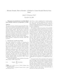
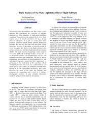
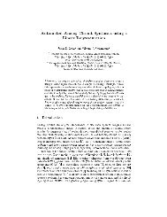
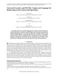
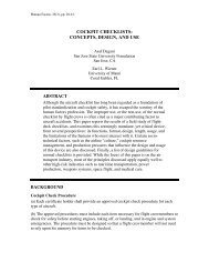
2. Each agent picks its choice of state according to theprobability distribution for L times sequentially, whereL is the Monte Carlo block size. We denote the numberof state x i picked by agent i by L xi . We require L xito be non-empty for all x i ∈ ω i , i.e., if some L xi = 0,we randomly pick a sample x ′ and set x i = x ′ i so thatL xi = 1. This process is to ensure that we can getconditional expected values [G|x i ] for all x i ∈ σ i . Itshould be noted though that it violates the assumptionsof IID sampling underpinning the derivation of the privateutilities minimizing bias plus variance.3. The gradients for each individual component is calculatedbased on the L samples taken from the previousstep (c.f. eq. 9), and gradient descents are performedfor all i simultaneously. Since all probabilities must bepositive, for each component i, the magnitude of descentis halved if q i (x i ) is no longer positive for somex i .4. Repeat steps 2 and 3.In figure 1, we have shown a comparison of three differentways of doing the descent direction estimation in step 3above. Team game means that we use [G|x i ] to get the descentdirections, weighted Aristocratic Utility correspondsto using the formula in eq. 12 to get the descent directions,and uniform Aristocratic Utility corresponds to simplifyingthe functions {g i } toĝ i (x) := G(x) − 1|σ i |∑x i∈σ iG(x −i , x i ). (14)dx ′ i L−1 x ′ iIn figure 1, we see that weighted AU outperforms uniformAU except at β −1 = 0.2. This unexpected result atβ −1 = 0.2 may be due to the limitation on the size of L.(Recall that we have required that L xi ≠ 0, and if it everdoes, we randomly pick a sample x ′ and set x i = x ′ i sothat L xi = 1.) Hence, as shown in figure 3, the numberof L xi = 1 is greater when β −1 = 0.2 than that whenβ −1 = 0.6. This demonstrates that at β −1 = 0.2, quite afew redistributions of the samples are happening and hencethe size of L has to be enlarged to get decent statistics.The speculation is further strengthened by comparing correctWLU (where−1x L∫ idefining agent i’s AU are replacedwith a delta function about about the least likely (accordingto q i ) of that agent’s moves) and incorrect WLU(where the same quantities are replaced with a delta functionabout about the most likely (according to q i ) of thatagent’s moves) with different sample size L. As shown infigures 4 and 5, the increase in sample size does amend theproblem caused by resampling.5. Unknown world utilitiesWe now consider the case where the explicit formula forthe world utility is not known and hence the calculations forWLU, uniform AU and weighted AU are not possible. Recallthat for this case we require that each player not onlysubmits her choices of actions during each Monte Carloblock, but her probability distribution as well. Although thisbrings a constant overhead to the transmission, this becomesnegligible when L is large.The problem we consider here is a 100-agent 4-night barproblem [14]. In this problem, each agent’s strategy set consistsof four elements: {1, 2, 3, 4}. The world utility is of theform:4∑G(x) = −50 × e −f k(x)/6(15)k=1where f k (x) = ∑ i δ(x i − k), i.e., f k (x) is the number ofagents attending the bar at night k. The precise algorithm isas follows:1. Each agent possesses a probability distribution on herset of actions: {q i (x i ) | x i ∈ ω i }, which is initially setto be uniform.2. Each agent picks its state according to the probabilitydistribution for L times sequentially, where L is theMonte Carlo block size, as well as her probability distribution{q i (x i ) | x i ∈ ω i }. Again, we require L xi tobe non-empty for all x i ∈ ω i , i.e., if some L xi = 0,we randomly pick a sample x ′ and set x i = x ′ i so thatL xi = 1.3. Denote the set of samples in the L Monte Carlo step byS, each agent generates a set of artificial data points accordingto agents’ probability distributions, and denotethose by A i . Then we define the following quantity:Ḡ xi := 1 − α ∑δ(x i − x ′|S|i)G(x) (16)x ′ ∈S+ α ∑δ(x i − x ′|A i |i)ĜS(x) (17)x ′ ∈A iwhere α is a weighting parameter between 0 and 1 andĜ is defined by:∑xĜ S (x) :=′ ∈S d(x, x′ )G(x ′ )∑x ′ ∈S d(x, (18)x′ )where d( . , . ) is some appropriate metric. In thepresent 100-agent 4-night bar problem, d(x, x ′ ) :=e −2×∑ 4|f k(x)−f k (x ′ )| k=1 where the functions {f k (.)}are as defined in eq. 15.4. Each agent updates her probability distribution accordingto the gradients calculated as in eq. 9 but with[G|x i ] replaced by Ḡx i. Again, for each agent i, the

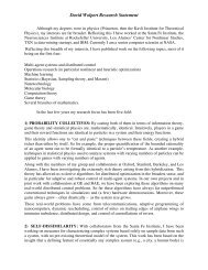
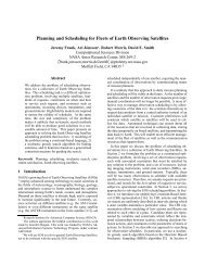
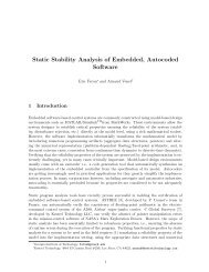
−30−40−50−60−70−80−900 0.5 1 1.5Figure 1. Plots of β −1 vs. the Lagrangianfor different utilities. The curves are generatedby plotting the Lagrangian at the 20thtimestep, i.e., after 20 descents. The initialstep sizes are set to be 0.2 times the gradients.Also, L = 100 and a total of 40 simulationsare performed. (Red dotted line: Teamgame, green dashed line: uniform AU, bluesolid line: weighted AU.)−30−35−40−45−500 5 10 15 20 25Figure 2. The time series of Lagrangian alongthe 20 time steps (curves generated at β −1 =0.6). (Red dotted line: Team game, greendashed line: uniform AU, blue solid line:weighted AU.)1.5magnitude of descent is halved if q i (x i ) is no longerpositive for some x ′ i .5. Repeat steps 2 to 4.Given that the utility function is reasonably smooth, itis natural to expect that the estimates aided by artificialdata points will provide an improvement. And this is indeedshown in figure 6 with varying α. The same experimentsare also performed for the 50-spin model introduced in section4.1 but with a new metric d(x, x ′ ) = ∑ 50i=1 δ(x i − x ′ i ).The results are shown in figure 7.An immediately improvement to the scheme above is torealize that there is no need to restrict ourselves to dataavailable in that particular time step in calculating Ḡx iineq. 16. Namely, unlike step 3 above, we can accumulate“true” data from previous steps in calculating Ḡx iwhichwill certainly improve the accuracy of the estimation. To illustratethis idea, at time step t, we define S ′ to be the settrue samples drawn at time step t and with the set of truesamples drawn at time step t − 1, and we calculate Ḡx ias:Ḡ xi := 1 − α|S|+ α|A i |∑δ(x i − x ′ i)G(x) (19)x ′ ∈S∑δ(x i − x ′ i)ĜS ′(x) . (20)x ′ ∈A iThe results for the bar problem are shown in figure 8.10.500 5 10 15 20 25Figure∑ ∑3. Plots of time step versus150 i x i ∈σ iδ(L xi − 1) at different temperatures.(Red dotted line: β −1 = 0.2, bluesolid line: β −1 = 0.6.)6. ConclusionProduct Distribution (PD) theory is a recently introducedbroad framework for analyzing, controlling, and optimizingdistributed systems [9, 10, 11]. Here we investigate PD theory’suse for adaptive, distributed control of a MAS. Typicallysuch control is done by having each agent run its ownreinforcement learning algorithm [4, 13, 14, 12].In this approach the utility function of each agent isbased on the world utility G(x) mapping the joint move of

−10−150−15−200−20−250−25−300 5 10 15Figure 4. The time series of Lagrangian alongthe 20 time steps with sample size L = 100(curves generated at β −1 = 0.2). (Red dottedline: correct WLU, blue solid line: incorrectWLU.)−3000 0.5 1 1.5Figure 6. Plots of β −1 vs. the Lagrangian withvarious weighing parameters α for the barproblem. The curves are generated by plottingthe Lagrangian at the 20th timestep. (Reddotted line: no data augmentation, greendashed line: data aug. with α = 0.3, blue solidline: data aug. with α = 0.5, black dashed dottedline: data aug. with α = 0.7.)−10−15−20−25−30−35−400 5 10 15 20 25Figure 5. The time series of Lagrangian alongthe 20 time steps with sample size L = 200(curves generated at β −1 = 0.2). (Red dottedline: correct WLU, blue solid line: incorrectWLU.)−20−30−40−50−60−70−800 0.5 1 1.5Figure 7. Plots of β −1 vs. the Lagrangianfor the 50-spin model. The curves are generatedby plotting the Lagrangian at the 20thtimestep. (Red dotted line: no data augmentation,blue solid line: data aug. with α = 0.5.)

−100−150−200−2500 0.5 1 1.5Figure 8. Plots of β −1 vs. the Lagrangianwith data accumulation (blue line) and withoutdata accumulation (red dotted line) forthe bar problem. The curves are generatedby plotting the free energies at the 10thtimestep. The initial step sizes are set to be0.2 times the gradients. Also, the number oftrue data |S| is 20, the number of data storedis 20 and the number of artificial data |A i | is40. A total of 80 simulations are performed.the agents, x ∈ X, to the performance of the overall system.However in practice the agents in a MAS are bounded rational.Moreover the equilibrium they reach will typically involvemixed strategies rather than pure strategies, i.e., theydon’t settle on a single point x optimizing G(x). This suggestsformulating an approach that explicitly accounts forthe bounded rational, mixed strategy character of the agents.PD theory directly addresses these issues by casting thecontrol problem as one of minimizing a Lagrangian of thejoint probablity distribution of the agents. This allows theequilibrium to be found using gradient descent techniques.In PD theory, such gradient descent can be done in a distributedmanner.We present experiments validating PD theory’s predictionsfor how to speed the convergence of that gradient descent.We then present other experiments validating the useof PD theory to improve convergence even if one is not allowedto rerun the system (an approach common in RLbasedschemes). These results demonstrate the power of PDtheory for providing a principled way to control a MAS ina distributed manner.References[1] S. Airiau and D. H. Wolpert. Product distribution theory andsemi-coordinate transformations. 2004. Submitted to AA-MAS 04.[2] N. Antoine, S. Bieniawski, I. Kroo, and D. H. Wolpert. Fleetassignment using collective intelligence. In Proceedings of42nd Aerospace Sciences Meeting, 2004. AIAA-2004-0622.[3] S. Bieniawski and D. H. Wolpert. Adaptive, distributed controlof constrained multi-agent systems. 2004. Submitted toAAMAS 04.[4] R. H. Crites and A. G. Barto. Improving elevator performanceusing reinforcement learning. In D. S. Touretzky,M. C. Mozer, and M. E. Hasselmo, editors, Advances in NeuralInformation Processing Systems - 8, pages 1017–1023.MIT Press, 1996.[5] D. Fudenberg and D. K. Levine. The Theory of Learning inGames. MIT Press, Cambridge, MA, 1998.[6] D. Fudenberg and J. Tirole. Game Theory. MIT Press, Cambridge,MA, 1991.[7] D. Mackay. Information theory, inference, and learning algorithms.Cambridge University Press, 2003.[8] S. Bieniawski W. Macready and D.H. Wolpert. Adaptivemulti-agent systems for constrained optimization. 2004.Submitted to AAAI 04.[9] D. H. Wolpert. Factoring a canonical ensemble. 2003. condmat/0307630.[10] D. H. Wolpert. Bounded rational games, information theory,and statistical physics. In D. Braha and Y. Bar-Yam, editors,Complex Engineering Systems, 2004.[11] D. H. Wolpert. Generalizing mean field theory for distributedoptimization and control. 2004. Submitted.[12] D. H. Wolpert and K. Tumer. Optimal payoff functionsfor members of collectives. Advances in Complex Systems,4(2/3):265–279, 2001.[13] D. H. Wolpert and K. Tumer. Collective intelligence, datarouting and braess’ paradox. Journal of Artificial IntelligenceResearch, 2002.[14] D. H. Wolpert, K. Wheeler, and K. Tumer. Collective intelligencefor control of distributed dynamical systems. EurophysicsLetters, 49(6), March 2000.Acknowledgements CFL thanks NASA and NSERC(Canada) for financial support.