Product distribution theory for control of multi-agent systems

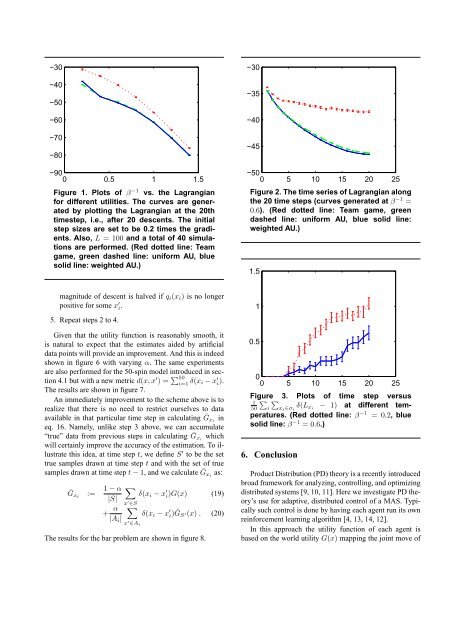
−30−40−50−60−70−80−900 0.5 1 1.5Figure 1. Plots of β −1 vs. the Lagrangianfor different utilities. The curves are generatedby plotting the Lagrangian at the 20thtimestep, i.e., after 20 descents. The initialstep sizes are set to be 0.2 times the gradients.Also, L = 100 and a total of 40 simulationsare performed. (Red dotted line: Teamgame, green dashed line: uniform AU, bluesolid line: weighted AU.)−30−35−40−45−500 5 10 15 20 25Figure 2. The time series of Lagrangian alongthe 20 time steps (curves generated at β −1 =0.6). (Red dotted line: Team game, greendashed line: uniform AU, blue solid line:weighted AU.)1.5magnitude of descent is halved if q i (x i ) is no longerpositive for some x ′ i .5. Repeat steps 2 to 4.Given that the utility function is reasonably smooth, itis natural to expect that the estimates aided by artificialdata points will provide an improvement. And this is indeedshown in figure 6 with varying α. The same experimentsare also performed for the 50-spin model introduced in section4.1 but with a new metric d(x, x ′ ) = ∑ 50i=1 δ(x i − x ′ i ).The results are shown in figure 7.An immediately improvement to the scheme above is torealize that there is no need to restrict ourselves to dataavailable in that particular time step in calculating Ḡx iineq. 16. Namely, unlike step 3 above, we can accumulate“true” data from previous steps in calculating Ḡx iwhichwill certainly improve the accuracy of the estimation. To illustratethis idea, at time step t, we define S ′ to be the settrue samples drawn at time step t and with the set of truesamples drawn at time step t − 1, and we calculate Ḡx ias:Ḡ xi := 1 − α|S|+ α|A i |∑δ(x i − x ′ i)G(x) (19)x ′ ∈S∑δ(x i − x ′ i)ĜS ′(x) . (20)x ′ ∈A iThe results for the bar problem are shown in figure 8.10.500 5 10 15 20 25Figure∑ ∑3. Plots of time step versus150 i x i ∈σ iδ(L xi − 1) at different temperatures.(Red dotted line: β −1 = 0.2, bluesolid line: β −1 = 0.6.)6. ConclusionProduct Distribution (PD) theory is a recently introducedbroad framework for analyzing, controlling, and optimizingdistributed systems [9, 10, 11]. Here we investigate PD theory’suse for adaptive, distributed control of a MAS. Typicallysuch control is done by having each agent run its ownreinforcement learning algorithm [4, 13, 14, 12].In this approach the utility function of each agent isbased on the world utility G(x) mapping the joint move of