Product distribution theory for control of multi-agent systems

More documents

Recommendations

Info

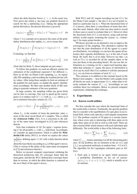
where the delta function forces x ′ i = x i in the usual way.Now given any initial q, one may use gradient descent tosearch for the q optimizing L(q). Taking the appropriatepartial derivatives, the descent direction is given by△q i (x i ) =δLδq i (x i ) = [G|x i] + β −1 log q(x i ) + C (9)where C is a constant set to preserve the norm of the probabilitydistribution after update, i.e., set to ensure that∫∫dx i q i (x i ) = dx i (q i (x i ) + △q i (x i )) = 1. (10)Evaluating, we find thatC = −∫ 1 ∫}dx i{[G|x i ] + β −1 log q i (x i ) . (11)dxi 1(Note that for finite X, those integrals are just sums.)To follow this gradient, we need an efficient scheme forestimation of the conditional expected G for different x i .Here we do this via Monte Carlo sampling, i.e., by repeatedlyIID sampling q and recording the resultant private utilityvalues. After using those samples to form an estimate ofthe gradient for each agent, we update the agents’ distributionsaccordingly. We then start another block of IID samplingto generate estimates of the next gradients.In large systems, the sampling within any given blockcan be slow to converge. One way to speed up the convergenceis to replace each [G | x i ] with [g i | x i ], where g i isset to minimize bias plus variance [9, 11]:∫g i (x) := G(x) −dx iL −1x i∫dx′i L −1x ′ iG(x −i , x i ), (12)where L xi is the number of times the particular value x iarose in the most recent block of L samples. This is calledthe Aristocrat Utility (AU). It is a correction to the utilityof the same name investigated in [13] and referencestherein.Note that evaluation of AU for agent i requires knowingG for all possible x i , with x (i) held fixed. Accordingly,we consider an approximation, which is called the WonderfulLife utility (WLU), in which we replace the valuesL −1x∫ idefining agent i’s AU with a delta function aboutdx ′ i L−1 x ′ iabout the least likely (according to q i ) of that agent’s moves.(This is version of the utility of the same name investigatedin [13] and references therein.)Below we present computer experiments validating thetheoretical predictions that AU converges faster than theteam game, and that the WLU defined here converges fasterthan its reverse, in which the delta function is centered onthe most likely of the agent’s moves.Both WLU and AU require recording not just G(x) forthe Monte Carlo sample x, but also G at a set of points relatedin a particular way to x. When the functional form ofG is known, often there is cancellation of terms that obviatesthis need. Indeed, often what one does need to recordin these cases is easier to evaluate than is G. However whenthe functional form of G is not known, using such privateutilities would require rerunning the system, i.e., evaluatingG for many points besides x.PD theory provides us an alternative way to improve theconvergence of the sampling. This alternative exploits thefact that the joint distribution of all the agents is a productdistribution. Accordingly, we can have the agents all announcetheir separate distributions {q i } at the end of eachblock. By itself, this is of no help. However say that x aswell as G(x) is recorded for all the samples taken so far(not just those in the preceding block). We can use this informationas a training set for a supervised learning algorithmthat estimates G. Again, this piece of information isof no use by itself. But if we combine it with the announced{q i }, we can form an estimate of each [G | x i ].This estimate is in addition to the estimate based on theMonte Carlo samples — here the Monte Carlo samples fromall blocks are used, to approximate G(x), rather than to directlyestimate the various [G | x i ]. Accordingly we cancombine these two estimates. Below we present computerexperiments validating this technique.4. Experiments4.1. Known world utilitiesWe first consider the case where the functional form ofthe world utility is known. Technically, the specific problemthat we consider is the equilibration of a spin glass in an externalfield, where each spin has a total angular momentum3/2. The problem consists of 50 spins in a circular formation,where every spin is interacting with three spins on itsright, three spins on its left as well as with itself. There arealso external fields which interact with each individual spindifferently. The world utility is thus of the following form:G(x) = ∑ h i x i + ∑J ij x i x j , (13)iwhere ∑ means summing over all the interacting pairsonce. In our problem, the set elements in the set {h i } and{J ij } are generated uniformly at random from −0.5 to 0.5.The algorithm for the Lagrangian estimation goes as follows:1. Each spin is treated as an agent which possessesa probability distribution on his set of actions:{q i (x i ) | x i ∈ σ i ≡ {−1, 1}}, which is initially set tobe uniform.
2. Each agent picks its choice of state according to theprobability distribution for L times sequentially, whereL is the Monte Carlo block size. We denote the numberof state x i picked by agent i by L xi . We require L xito be non-empty for all x i ∈ ω i , i.e., if some L xi = 0,we randomly pick a sample x ′ and set x i = x ′ i so thatL xi = 1. This process is to ensure that we can getconditional expected values [G|x i ] for all x i ∈ σ i . Itshould be noted though that it violates the assumptionsof IID sampling underpinning the derivation of the privateutilities minimizing bias plus variance.3. The gradients for each individual component is calculatedbased on the L samples taken from the previousstep (c.f. eq. 9), and gradient descents are performedfor all i simultaneously. Since all probabilities must bepositive, for each component i, the magnitude of descentis halved if q i (x i ) is no longer positive for somex i .4. Repeat steps 2 and 3.In figure 1, we have shown a comparison of three differentways of doing the descent direction estimation in step 3above. Team game means that we use [G|x i ] to get the descentdirections, weighted Aristocratic Utility correspondsto using the formula in eq. 12 to get the descent directions,and uniform Aristocratic Utility corresponds to simplifyingthe functions {g i } toĝ i (x) := G(x) − 1|σ i |∑x i∈σ iG(x −i , x i ). (14)dx ′ i L−1 x ′ iIn figure 1, we see that weighted AU outperforms uniformAU except at β −1 = 0.2. This unexpected result atβ −1 = 0.2 may be due to the limitation on the size of L.(Recall that we have required that L xi ≠ 0, and if it everdoes, we randomly pick a sample x ′ and set x i = x ′ i sothat L xi = 1.) Hence, as shown in figure 3, the numberof L xi = 1 is greater when β −1 = 0.2 than that whenβ −1 = 0.6. This demonstrates that at β −1 = 0.2, quite afew redistributions of the samples are happening and hencethe size of L has to be enlarged to get decent statistics.The speculation is further strengthened by comparing correctWLU (where−1x L∫ idefining agent i’s AU are replacedwith a delta function about about the least likely (accordingto q i ) of that agent’s moves) and incorrect WLU(where the same quantities are replaced with a delta functionabout about the most likely (according to q i ) of thatagent’s moves) with different sample size L. As shown infigures 4 and 5, the increase in sample size does amend theproblem caused by resampling.5. Unknown world utilitiesWe now consider the case where the explicit formula forthe world utility is not known and hence the calculations forWLU, uniform AU and weighted AU are not possible. Recallthat for this case we require that each player not onlysubmits her choices of actions during each Monte Carloblock, but her probability distribution as well. Although thisbrings a constant overhead to the transmission, this becomesnegligible when L is large.The problem we consider here is a 100-agent 4-night barproblem [14]. In this problem, each agent’s strategy set consistsof four elements: {1, 2, 3, 4}. The world utility is of theform:4∑G(x) = −50 × e −f k(x)/6(15)k=1where f k (x) = ∑ i δ(x i − k), i.e., f k (x) is the number ofagents attending the bar at night k. The precise algorithm isas follows:1. Each agent possesses a probability distribution on herset of actions: {q i (x i ) | x i ∈ ω i }, which is initially setto be uniform.2. Each agent picks its state according to the probabilitydistribution for L times sequentially, where L is theMonte Carlo block size, as well as her probability distribution{q i (x i ) | x i ∈ ω i }. Again, we require L xi tobe non-empty for all x i ∈ ω i , i.e., if some L xi = 0,we randomly pick a sample x ′ and set x i = x ′ i so thatL xi = 1.3. Denote the set of samples in the L Monte Carlo step byS, each agent generates a set of artificial data points accordingto agents’ probability distributions, and denotethose by A i . Then we define the following quantity:Ḡ xi := 1 − α ∑δ(x i − x ′|S|i)G(x) (16)x ′ ∈S+ α ∑δ(x i − x ′|A i |i)ĜS(x) (17)x ′ ∈A iwhere α is a weighting parameter between 0 and 1 andĜ is defined by:∑xĜ S (x) :=′ ∈S d(x, x′ )G(x ′ )∑x ′ ∈S d(x, (18)x′ )where d( . , . ) is some appropriate metric. In thepresent 100-agent 4-night bar problem, d(x, x ′ ) :=e −2×∑ 4|f k(x)−f k (x ′ )| k=1 where the functions {f k (.)}are as defined in eq. 15.4. Each agent updates her probability distribution accordingto the gradients calculated as in eq. 9 but with[G|x i ] replaced by Ḡx i. Again, for each agent i, the
Page 1 and 2: Product distribution theory for con
Page 3: = ∑ i∫β i [dx ∏ jq j (x j )g
Page 7 and 8: −10−150−15−200−20−250

Product distribution theory for control of multi-agent systems

You also want an ePaper? Increase the reach of your titles

Delete template?

Save as template?