Mixture Density Mercer Kernels - Intelligent Systems Division - NASA

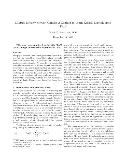
Mixture Density Mercer Kernels: A Method to Learn Kernels Directly fromData ∗Ashok N. Srivastava, Ph.D. †December 29, 2003This paper was submitted to the 2004 SIAMData Mining Conference on September 15, 2003.AbstractThis paper presents a method of generating Mercer Kernelsfrom an ensemble of probabilistic mixture models,where each mixture model is generated from a Bayesianmixture density estimate. We show how to convert theensemble estimates into a Mercer Kernel, describe theproperties of this new kernel function, and give examplesof the performance of this kernel on unsupervisedclustering of synthetic data and also in the domain ofunsupervised multispectral image understanding.Keywords: Clustering, Mixture Density Estimation,Kernel Methods, Unsupervised Learning, Image Segmentation1 Introduction and Previous WorkThis paper addresses the problem of estimating theposterior probability of a continuous random variablex ∈ R d assuming that the underlying data generatingprocess is possibly a Gaussian mixture density function.The posterior probability we wish to estimate is P (c|x i )where x i is one of N independent and identicallydistributed realizations from a data set X and c is oneof C clusters or modes. There is an abundant literatureon mixture density estimation, as it arises in classicalstatistics [12], statistical machine learning [8], and datamining [2]. Recently, there has been additional workin performing clustering [7] or density estimation [11]in high, possibly infinite dimensional Hilbert spacesdefined by Mercer Kernels.Traditional algorithms used to generate the probabilitydensity P (x|Θ) assume that:(1.1)P (x|Θ) =C∑P (c)P (x|θ c )c=1∗ This work is funded in part by NASA’s Intelligent DataUnderstanding program.† Research Institute of Advanced Computer Science, NASAAmes Research Centerwhere Θ is a vector containing the C model parameters,and θ c are the model parameters for the cth mixturecomponent. The parameters of such a model areobtained through Expectation Maximization of the appropriatelog-likelihood function or, more generally, theposterior log-likelihood.We propose to assess the posterior class probabilitiesby generating a kernel function K(x i , x j ) that measuresthe similarity between two data points x i and x jthrough the use of an ensemble of mixture densities ofthe form given above. We show that under certain simplifyingconditions this kernel function, which we calla mixture density kernel is a Gram matrix that measuresthe number of times on average an ensemble ofmixture density estimates agree that two points arisefrom the same mode of the probability density function.This kernel function capitalizes on the fact thateach estimated probability density function is a nonoptimalsample from a model space, and relies heavilyon the theory of bagged classifiers [1]. We also showthat the ensemble of mixture models is a method toempirically combine the posterior probabilities, and relationsto the theory of kernel alignment are given. Dueto the fact that the kernel function can be derived froman ensemble of Bayesian mixture models, we have theability to encode domain knowledge in the kernel functionthrough the use of informative priors, thus aidingthe search for an optimal model. Although this paperpresents results of this kernel function on unsupervisedlearning problems, they can be applied equally well totypical supervised learning learning problems such asclassification and regression in a straightforward manner.The paper begins with a description of the notationused in this paper, gives a brief introduction to Bayesianmixture modelling, introduces Mercer kernels and showshow they can be interpreted as a similarity measure,introduces Mixture Density Kernels and compares themwith other kernel functions, and then gives experimentalresults of the algorithm on unsupervised learning ina synthetic data set and then a real-world task ofmultispectral image understanding.

2 Notation• p is the dimension of the data• M is the space of models from which the mixturedensity models are drawn.• F is the feature space, which may be a highdimensional (but finite) space, or more generallyan infinite dimensional Hilbert space.• N is the number of data points x i drawn from a pdimensional space• M is the number of probabilistic models used ingenerating the kernel function.• C is the number of mixture components in eachprobabilistic model. In principle one can use adifferent number of mixture components in eachmodel. However, here we choose a fixed numberfor simplicity.• x i is a p × 1 dimensional real column vector thatrepresents the data sampled from a data set X .• Φ(x) : R p ↦→ F is generally a nonlinear mappingto a high, possibly infinite dimensional, featurespace F. This mapping operator may be explicitlydefined or may be implicitly defined via a kernelfunction.• K(x i , x j ) = Φ(x i )Φ T (x j ) ∈ R is the kernelfunction that measures the similarity between datapoints x i and x j . If K is a Mercer kernel, it canbe written as the outer product of the map Φ.As i and j sweep through the N data points, itgenerates an N × N kernel matrix.• Θ is the entire set of parameters that specify amixture model.3 Mixture Models: A Sample from a ModelSpaceIn this section, we briefly motivate the development ofMixture Density Kernels by showing that the combinedresult of model misspecification and the effects of a finitedata set can lead to high uncertainty in the estimate ofa mixture model. We closely follow the arguments givenin [15].Suppose that a data set X is generated by drawing afinite sample from a mixture density function f(Λ ∗ , Θ ∗ ),where Λ ∗ defines the true density function (say a Gaussianmixture density) and is a sample from a large butfinite class of models M, and Θ ∗ defines the true setof parameters of that density function. In the case ofthe Gaussian mixture density, these parameters wouldbe the means and covariance matrices for each Gaussiancomponent, and the number of components thatcomprise the model. We can compute the probabilityof obtaining the correct model given the data as follows(see Smyth and Wolpert, 1998 for a detailed discussion).The posterior probability of the true densityf ∗ ≡ f(Λ ∗ , Θ ∗ ) given the data X is:∫ ∫P (f(Λ ∗ , Θ ∗ )|X ) =P (Λ, Θ|X ) ×MR(M)δ(f ∗ − P (Λ, Θ))dΛdΘwhere the first integral is taken over the model spaceM and the second integral is taken over the region inthe parameter space that is appropriate for the modelΛ, and δ is the Dirac delta function. Using Bayes rule,it is possible to expand the posterior into a product ofthe posterior of the model uncertainty and the posteriorof the parameter uncertainty. Thus, we have:∫ ∫P (f ∗ |X ) =P (Λ|X )P (Θ|Λ, X ) ×=MR(M)δ(f ∗ − P (Λ, Θ))dΛdΘ∫ ∫1P (Θ|Λ, X )P (Λ, X ) ×P (X )MR(M)δ(f ∗ − P (Λ, Θ))dΛdΘThe first equation above shows that there are twosources of variation in the estimation of the densityfunction. The first is due to model misspecification, andthe second is due to parameter uncertainty. The secondequation shows that if prior information is available, itcan be used to modify the likelihood of the data in orderto obtain a better estimate of the true density function.The goal of this paper is to seek a representationof the posterior P (x i |Θ) by reducing these errors byembedding x i in a high dimensional feature space thatdefines a kernel function.4 Review of Kernel FunctionsMercer Kernel functions can be viewed as a measureof the similarity between two data points that are embeddedin a high, possibly infinite dimensional featurespace. For a finite sample of data X , the kernel func-

tion yields a symmetric N × N positive definite matrix,where the (i, j) entry corresponds to the similaritybetween (x i , x j ) as measured by the kernel function.Because of the positive definite property, such a MercerKernel can be written as the outer product of thedata in the feature space. Thus, if Φ(x i ) : R d ↦→ Fis the (perhaps implicitly) defined embedding function,we have K(x i , x j ) = Φ(x i )Φ T (x j ). Typical kernel functionsinclude the Gaussian kernel for which K(x i , x j ) =Φ(x i )Φ T (x j ) = exp(− 12σ 2 ||x i − x j || 2 ), and the polynomialkernel K(x i , x j ) = Φ(x i )Φ T (x j ) =< x i , x j > p .For supervised learning tasks, linear algorithms areused to define relationships between the target variableand the embedded features [4]. Work has also been donein using kernel methods for unsupervised learning tasks,such as clustering [7, 16] and density estimation [11].5 Mixture Density KernelsThe idea of using probabilistic kernels was discussedby Haussler in 1999 [9] where he observesthat∑if K(x i , x j ) ≥ 0 ∀ (x i , x j ) ∈ X × X , and∑x i x jK(x i , x j ) = 1 then K is a probability distributionand is called a P-Kernel. He further observedthat the Gibbs kernel K(x i , x j ) = P (x i )P (x j ) is alsoan admissible kernel function.Although these kernel functions either represent orare derived from probabilistic models, they may notmeasure similarity in a consistent way. For example,suppose that x i is a low probability point, so thatP (x i ) ≈ 0, In the case of the Gibbs kernel, K(x i , x i ) ≈0, although the input vectors are identical. The Grammatrix generated by this kernel function would onlyshow those points as being similar which have very highprobabilities. While this feature may be of value insome applications, it needs modification to work as asimilarity measure.Our idea is to use an ensemble of probabilistic mixturemodels as a similarity measure. Two data pointswill have a larger similarity if multiple models agreethat they should be placed in the same cluster or modeof the distribution. Those points where there is disagreementwill be given intermediate similarity measures.The shapes of the underlying mixture distributionscan significantly affect the similarity measurementof the two points. Experimental results uphold this intuitionand show that in regions where there is “no question”about the membership of two points, the MixtureDensity Kernel behaves identically to a standardmixture model. However, in regions of the input spacewhere there is disagreement about the membership oftwo points, the behavior may be quite different thanthe standard model. Since each mixture density modelin the ensemble can be encoded with domain knowledgeby constructing informative priors, the Bagged ProbabilisticKernel will also encode domain knowledge. TheBagged Probabilistic Kernel is defined as follows:K(x i , x j ) = Φ(x i )Φ T (x j )=1M∑Z(x i , x j )C m∑m=1 c m =1P m (c m |x i )P m (c m |x j )The feature space is thus defined explicitly as follows:Φ(x i ) = [P 1 (c = 1|x i ), P 1 (c = 2|x i ), . . . ,P 1 (c = C|x i ), P 2 (c = 1|x i ), . . . , P M (c = C|x i )]The first sum in the defining equation above sweepsthrough the M models in the ensemble, where eachmixture model is a Maximum A Posteriori estimatorof the underlying density trained by sampling (withreplacement) the original data. We will discuss howto design these estimators in the next section. C mdefines the number of mixtures in the mth ensemble,and c m is the cluster (or mode) label assigned by themodel. The quantity Z(x i , x j ) is a normalization suchthat K(x i , x i ) = 1 for all i. The fact that the MixtureDensity Kernel is a valid kernel function arises directlyfrom the definition. In order to prove K is a valid kernelfunction, we need to show that it is symmetric, and thatthe kernel matrix is positive semi-definite[4]. The kernelis clearly symmetric since K(x i , x j ) = K(x j , x i ) for allvalues of i and j. The proof that K is positive semidefiniteis straightforward and arises from the fact thatΦ can be explicitly known. For nonzero α:(5.2)α T K(x i , x j )α = α T Φ(x i )Φ T (x j )α = β T β ≥ 0The Mixture Density Kernel function can be interpretedas follows. Suppose that we have a hard classificationstrategy, where each data point is assigned to themost likely posterior class distribution. In this case thekernel function counts the the number of times the Mmixtures agree that two points should be placed in thesame cluster mode. In the soft classification strategy,two data points are given an intermediate level of similaritywhich will be less than or equal to the case whereall models agree on their membership. Further interpretationof the kernel function is possible by applyingBayes rule to the defining equation of the Mixture DensityKernel. Thus, we have:(5.3)K(x i , x j ) ==M∑C m∑m=1 c m =1P m (x i |c m )P m (c m )P m (x i )×P m (x j |c m )P m (c m )P m (x j )M∑ ∑C mP m (x i , x j |c m )Pm(c 2 m )P m (x i , x j )m=1 c m =1

The second step above is valid under the assumptionthat the two data points are independent and identicallydistributed. This equation shows that the Mixture DensityKernel measures the ratio of the probability thattwo points arise from the same mode, compared withthe unconditional joint distribution. If we simplify thisequation further by assuming that the class distributionsare uniform, the kernel tells us on average (acrossensembles) the amount of information gained by knowingthat two points are drawn from the same mode in amixture density.It is not possible to obtain similarity through computingthe average density across an ensemble (whichwould be the traditional approach to bagging), becausein that case, P (x) = ∑ M ∑ Km=1 k=1 P m(k|x)P m (k) the assignmentof a data point to a given mixture componentis arbitrary. Thus, for two given probabilistic modelsP m and P n , cluster c m may not be the same as clusterc n . This lack of similarity may go beyond the mere problemthat the mixture assignments are arbitrary. Thegeometry of the mixture components may be differentfrom run to run. For example, in the case of a Gaussianmixture model, the positions of the mean vectors µ mand µ n and their associated covariance matrices maybe different.The dimension of the feature space defined by theBagged Probabilistic Kernel is large but finite. In thecase where the number of components varies for eachmember, the dimensionality is dim(F) = ∑ Mm=1 C m.Once normalized to unit length (through the factorZ(x i , x j )), the Φ(x i ) vectors represent points on ahigh dimensional hypersphere. The angle between thevectors determines the similarity between the two datapoints, and the (i, j) element of the kernel matrix is thecosine of this angle.Building the Mixture Density Kernel requires buildingan ensemble of mixture density models, each representinga sample from the larger model space M. Thegreater the heterogeneity of the models used in generatingthe kernel, the more effective the procedure. Inour implementation of the procedure, the training datais sampled M times with replacement. These overlappingdata sets, combined with random initial conditionsfor the EM algorithm, aid in generating a heterogenousensemble. Other ways of introducing heterogeneity includeencoding domain knowledge in the model. Thiscan be accomplished through the use of Bayesian MixtureDensities, which is the subject of the next section.6 Review of Bayesian Mixture DensityEstimationA Bayesian formulation to the density estimation problemrequires that we maximize the posterior distributionP (Θ|X ) which arises as follows:(6.4)P (Θ|X ) =P (X |Θ)P (Θ)P (X )Cheeseman and Stutz 1995, among others, showed thatprior knowledge about the data generating process canbe encoded in the prior P (Θ) in order to guide theoptimization algorithm toward a model Θ ′ that takesthe domain knowledge into account. This prior assumesthat a generative model Λ has been chosen (such asa Gaussian), and determines the prior over the modelparameters.A Bayesian formulation to the mixture densityproblem requires that we specify the model (Λ) and thena prior distribution of the model parameters. In thecase of a Gaussian mixture density model for x ∈ R d ,we take the likelihood function as:P (x|θ c ) = P (x|µ c , Σ c , c)= (2π) − d 2 |Σc | − 1 2 ×exp[− 1 2 (x − µ c) T Σ −1c (x − µ c )]In the event that domain information is to be encoded, itis convenient to represent it in terms of a conjugate priorfor the Gaussian distribution. A conjugate is defined asfollows:Definition 6.1. A family F of probability densityfunctions is said to be conjugate if for every f ∈ F ,the posterior f(Θ|x) also belongs to F .For a mixture of Gaussians model, priors can be set asfollows[6]:• For priors on the means, either a uniform distributionor a Gaussian distribution can be used.• For priors on the covariance matrices, theWishart density can be used: P (Σ i |α, β, J) ∝|Σ −1i | β 2 exp(−αtr(Σ −1 J)/2).i• For priors on the mixture weights, a Dirichletdistribution can be used: P (p i |γ) ∝ ∏ Cc=1 pγ i−1i ,where p i ≡ P (c = i).These priors can be viewed as regularizers for the mixturenetwork as in [14]. Maximum a posteriori estimationis performed by taking the log of the posteriorlikelihood of each data point x i given the model Θ. Thefollowing function is thus optimized using the ExpectationMaximization[5]:[ N]∏(6.5) l(Θ) = log P (x i |Θ)P (Θ)i=i

In some cases, details of the underlying distributionare known and can be used to influence the estimateddistribution. For example, in some cases there maybe prior knowledge of the class distribution based onprevious work, in which case the Dirichlet distributionwould be appropriate. Many studies can be performedusing noninformative priors, in which case P (Θ) ≡ 1.In the former case, the mixture density kernel takesdomain information into account, whereas in the lattercase, it is determined directly from the data.7 Comparison with Other KernelsWe now compare the Mixture Density Kernel with threeother types of kernels: the Gaussian or Radial BasisFunction (RBF) kernel and other parametric kernelssuch as the polynomial kernel, the Fisher kernel, andkernel alignment, where the functions are designed tomaximize the accuracy of a prediction.The RBF kernel and other parametric kernel functionsare usually chosen using some heuristic methodwhere the classification accuracy or other criterion isused to choose the best kernel. In the case of the MixtureDensity Kernel, the underlying structure of thedata is used to generate the kernel function. Thus, itcan improve upon the standard set of kernel functionsand can be used in situations where no clear objectivecriterion is available, such as in unsupervised learningproblems like clustering. The parametric kernels are appropriatefor use in unsupervised and supervised problemsalike.The Fisher kernel as developed by Jaakkola andHaussler (1999) [10] and the “Tangent of vectors ofposterior log odds” [17] kernel use probabilistic modelsto generate kernel functions. Kernel Alignment [3]is another method to generate kernel functions, butdoes not use a probabilistic model as its underlyingbasis. However, these kernel functions are optimized fordiscriminative performance and may not be appropriatefor unsupervised problems such as clustering.8 Kernel Clustering in Feature SpaceGirolami, (2001) has given an algorithm to performclustering in the feature space using an approach similarto k-means clustering. A brief review of the methodfollows. The cost function for k-means clustering in thefeature space at a given instant in time is:G Φ = 1 NN∑i=1 k=1[Φ(Z i ) − m Φ k ]K∑q ki [Φ(Z i ) − m Φ k ] T ×where q ki is the cluster membership indicator function(q ki = 1 if vector Z i is a member of cluster k, andzero otherwise), and m Φ kis the cluster center in the featurespace. Thus, if we expand the right-hand side ofthe above equation, and take m Φ k = 1 ∑ NN i=1 q kiΦ(Z i ),which represents the centroid of the cluster in featurespace, we obtain an equation in which only inner productsappear. The nonlinear mapping Φ does not needto be determined explicitly because the kernel functionis taken as the inner product in the feature space:K ij = Φ T (Z i )Φ(Z j ). The objective of kernel clusteringis to find a membership function q and cluster centersm Φ that minimize the cost G Φ . Various methods canbe used to minimize G Φ , including annealing methods(as described in Girolami, 2001) or direct search. Ifthe annealing method is used, the cluster centers areimplicitly defined. However, depending on the kernelfunction used, a direct search approach allows for thepre-image of the cluster center to be explicitly known.Note that K, the number of clusters in the feature space,need not be directly related to ∑ Mc=1 C m, which is thenumber of dimensions of the feature space, nor does Kneed to be a direct function of the number of modesin each mixture ensemble. After the optimization iscompleted, it is possible to compute the uncertainty inthe clustering by computing the entropy of the clusterassignment probability for a given point throughe(x i ) = − ∑ Kk=1 q ki log q ki . We use this quantity tocharacterize the quality of our results in subsequent experiments.9 Experiments and ResultsIn this section, we describe the performance of the MixtureDensity Kernels on a synthetic clustering problemand on a real-world image segmentation problem. Forthe synthetic data set, we show that the algorithm producessuperior results when compared with a standardGaussian kernel.9.1 Clustering with Mixture Density MercerKernels on Synthetic Data Figure 1 shows a plotof the two-dimensional synthetic data. These data aregenerated from a mixture of three Gaussians. Thefirst Gaussian, labelled with the symbol ’o’ has a smallvariance compared with the other two Gaussians. Thesecond Gaussian has a larger spread, and the thirdGaussian partially overlaps the first and second [13].We generated 10,000 points for training, testing, andevaluation of the model. We recognize that this amountof data is very large to specify the model, but wantedto also obtain an estimate of the performance of thealgorithm on a moderate sized data set.The first experiment consists of computing theKernel matrix for the synthetic data using a GaussianKernel as well as the Mixture Density Mercer Kernels.

Kernel Matrix for Mixture Density Mercer Kernel with Non−Informative PriorFigure 3: The kernel matrix generated from the MixtureDensity Mercer Kernels. While Class 1 continues to beclearly demarcated in the upper left hand region as withthe Gaussian Kernel, this kernel also does a better jobat distinguishing between Clusters 2 and 3. The meansquared error between the correct kernel matrix and theestimated kernel matrix is 0.04 ± 10%. Notice thatsome points are not correctly classified by this kernel asindicated by the dark vertical lines in the off-diagonalregions of the matrix. These lines correspond to pointsin the data space which arise from overlapping modesof the mixture density.segmentation problem. We begin by giving a briefmotivation of the problem, followed by an analysis ofthe results.The detection of clouds within a satellite imageis essential for retrieving surface geophysical parametersfrom optical and thermal imagery. Operationalsurface albedo and temperature products require thecloud-detection because the retrieval methods are validfor clear skies only. Even a small percentage of cloudcover within a radiometer pixel can affect in such away that determination of surface variables, such asalbedo and temperature becomes impossible. Thus, routineprocessing of satellite data requires reliable automatedcloud detection algorithms that are applicableto a wide range of surface types. Unfortunately, clouddetection,particularly over snow- and ice-covered surfacesis a problem that has plagued working with opticaland thermal imagery since the first satellite-imagingsensor. Cloud-detection over snow and ice is difficultdue to the lack of spectral contrast between clouds andsnow. However, spectral information in the shortwaveinfrared, texture patterns, and other features may beused together to detect cloud contamination.Common approaches to detecting cloud cover arebased on spectral contrast, radiance spatial contrast,radiance temporal contrast, or a combination of thesemethods. These techniques work well over dark targets(e.g. vegetation), since clouds appear brighter (higheralbedo) in the visible range, and have lower temperaturesin the infrared compared to the cloud-free background.Threshold values are then chosen to representthe cloud-free background. Problems with this methodhowever, are that different thresholds typically need tobe selected from scene to scene. Another type of clouddetection that does not require absolute thresholds evaluatesthe spatial coherence of the observed scene. However,coherence tests suffer from the fact that false detectionis likely for clear pixels directly adjacent to cloudpixels.10 Data and Experimental ResultsWe obtained MODIS level 1B data for the Greenland icesheet from the NASA Langley DAAC and mapped thedata to a 1.25 km equal-area scalable Earth-grid (EASEgrid)using software developed by NSIDC to processMODIS level 1B data and convert the visible channeldata to top-of-the-atmosphere (TOA) reflectances.Next the TOA reflectances were normalized by the cosineof the solar zenith angle. Only the first 7 MODISchannels were used for this study. The image shown inFigure 4 was taken on day 188 of the year 2002 andis the output of Channel 6, which is tuned to detectclouds. Figure 5 shows the corresponding test image,which was taken on day 167 of the year 2002. We areunable to show the images in the other 5 bands dueto space limitations. As expected, the spectral signalsfor the 7 different MODIS channels are highly correlated,with linear correlation coefficients over 98% Weused this data as a training set for the Mixture DensityMercer Kernel. We prepared the data for use in the algorithmby taking the first difference across the spectralbands thus yielding 6 differenced bands and then building5 × 5 blocks of the data. This procedure results ina 150 dimensional vector representing each pixel, where150 = 5×5×6. We have found that the differencing procedureyields improved results for the Mixture DensityKernel as well as for other detection algorithms.Figure 6 shows the result of learning a standardGaussian Mixture Model with 10 modes on the trainingdata in Figure 4, and applying that model to the testdata shown in Figure 5. The model does a good jobat segmenting the image, and reveals the large threeprongedcloud over the ice sheet. However, noticethat the cloud is characterized as a single monolithicentity with little structure depicted within it. A carefulcomparison of the same region with the test image in

Channel 6 Data0.60.5Channel Spectral Wavelength(nm)1 620-6702 841-8763 459-4794 545-5655 1230-12506 1628-16527 2105-21550.40.30.20.1Table 1: The bandwidths for the first seven MODISchannels. The spatial resolutions for Channels 1 and 2are 250 m, and 500 m for Channels 3-7.Figure 5: This figure shows the output of Channel 6 forday 167 in the year of 2002 from the MODIS instrument.Clouds are characterized by regions of greater density ofwhite. This data was used to test the Mixture DensityMercer Kernel as well as the Gaussian Mixture Model.Figure 4: This figure shows the output of Channel 6 forday 188 in the year of 2002 from the MODIS instrument.Clouds are characterized by regions of greater densityof white. This data was used for training the MixtureDensity Mercer Kernel as well as the Gaussian MixtureModel.0.60.50.40.30.20.1Figure 5 shows that there is considerable structure tothe cloud that is missed. Furthermore, other regions,such as the large cloud in the lower right hand portion ofthe image are broken into multiple constituents, whereasChannel 6 does not show such structure.Figure 7 shows the results of applying the same datato the Mixture Density Kernel. We built the kernel onthe same training data, and used 10 mixtures in eachmodel in the ensemble. We built 50 ensembles, resultingin a 500 dimensional feature space. The first area tonotice is the structure of the three-pronged cloud overthe ice sheet. This structure indicates that the cloud isnot a homogeneous entity, but has several constituents.The western side of the image also shows a considerableamount of variation, particularly in the clouds in thelower part of the image. We point out these detailsin contrast to the results for the Gaussian MixtureModel for the same region. These results suggest thatthe Mixture Density Kernel can reveal new featuresin the data in some cases better than the GaussianMixture Model. However, such variation can be foundin other regions of the image, thus making an objectiveevaluation difficult. This difficulty is not unique toMixture Density Kernels and applies equally to generalunsupervised learning algorithms.11 Discussion and ConclusionsWe have shown a method to generate a Mercer Kernelfunction from an ensemble of mixture models. The

GMM Result10Kernel Cluster Uncertainty0.25980.2760.1550.1430.052Figure 6: The results of applying a Gaussian MixtureModel to the test data using 10 mixture coefficients.This model does a good job at segmenting the imageacross the seven spectral bands. Notice that the largethree-pronged cloud is characterized as a single entity.1Figure 8: This figure shows the uncertainty in thecluster assignment as shown by the entropy of classdistribution. It is interesting to note that there is verylow uncertainty over most of the ice sheet, even thoughit is divided into two entities. The three-pronged cloudover the ice sheet shows up as a region with higheruncertainty, as one would expect.Kernel Cluster Result10Figure 7: This figure shows the results of the MixtureDensity Mercer Kernel on the test data using 10 mixturesin the ensemble with 50 models in total. In comparisonto the Gaussian Mixture Model, these resultsshow a difference in the characterization of the threeprongedcloud over the ice sheet. This cloud shows additionalstructure using two different elements. Otherareas of comparison are the three clouds at the top ofthe image. The Mixture Density Mercer Kernel methodcorrectly segments these into the same class, whereasthere is considerable variation in the competing model.987654321Mixture Density Mercer Kernel function is the dotproduct of the vectors of class distributions acrossensembles. We have shown that this function canbe interpreted as a new similarity measure betweentwo data points, and has the feature that regions ofhigher uncertainty can be reduced. We exhibited thealgorithm in an unsupervised clustering setting, whereit shows some promise. We have also shown that theMixture Density Mercer Kernel can incorporate domainknowledge through its inclusion as a prior distributionon the ensemble models. While the algorithm has someadvantages, it is expensive to compute and still exhibitssome run-to-run variation. We are currently researchingmethods to further reduce this variation.This paper has shown the behavior of the new kernelon unsupervised clustering problems. We are currentlypreparing the results of using this kernel function forsupervised prediction problems, in particular on thesnow, ice, and cloud classification.12 AcknowledgementsThe author would like to thank Bill Macready, NikunjOza, and Julienne Stroeve for valuable discussions andfeedback. Dr. Stroeve also provided the MODISdata used as examples in this paper. This work wassupported by the NASA Intelligent Data Understandingsegment of the Intelligent Systems Program.

References[1] L. Breiman, Bagging predictors, Machine Learning 26(1996), 123–140.[2] P. Cheeseman and J. Stutz, Bayesian classification(autoclass): Theory and results, Advances in KnowledgeDiscovery and Data Mining (1995).[3] N. Cristianini, J. Kandola, A. Elisseeff, and J. Shawe-Taylor, On kernel target alignment, Journal of MachineLearning Research (2002).[4] N. Cristianini and J. Shawe-Taylor, An introduction tosupport vector machines, Cambridge University Press,2000.[5] A. P. Dempster, M. Laird, N., and D. B. Rubin,Maximum likelihood from incomplete data via the emalgorithm, Journal of the Royal Statistical Society B(1977).[6] Operations for Learning with Graphical Models, Buntine,w. l., Journal of Artificial Intelligence Research 2(1994), no. 1, 159–225.[7] M. Girolami, Mercer kernel based clustering in featurespace, IEEE Transactions on Neural Networks 13(2001), no. 4, 780–784.[8] T. Hastie, R. Tibshirani, and J. Friedman, The elementsof statistical learning: Data mining, inference,and prediction, Springer, 2001.[9] D. Haussler, Convolution kernels on discrete structures,Tech. report, University of California SantaCruz, 1999.[10] T. Jaakkola and D. Haussler, Exploiting generativemodels in discriminative classifiers, Advances in NeuralInformation Processing Systems 11 (1999).[11] W. G. Macready, Density estimation with mercer kernels,Technical Report TR03.13 of the Research Instituteof Advanced Computer Science (2003).[12] K. V. Mardia, J. T. Kent, and J. M. Bibby, Multivariateanalysis, Academic Press, 1979.[13] I. T. Nabney, Netlab, (2001).[14] D. Ormoneit and V. Tresp, Improved gaussian mixturedensity estimates using bayesian penalty terms andnetwork averaging, Advances in Neural InformationProcessing Systems, vol. 8, 1995.[15] P. Smyth and D. Wolpert, Stacked density estimation,Advances In Neural Information Processing Systems10 (1998).[16] A. N. Srivastava and J. Stroeve, Onboard detectionof snow, ice, clouds, and other geophysical processesusing kernel methods, Proceedings of the ICML 2003Workshop on Machine Learning Technologies for AutonomousSpace Applications, 2003.[17] K. Tsuda, M. Kawanabe, G. Ratsch, S. Sonnenburg,and K.R. Muller, A new discriminative kernel fromprobabilistic models, Neural Computation (2002).