Mixture Density Mercer Kernels - Intelligent Systems Division - NASA

More documents

Recommendations

Info

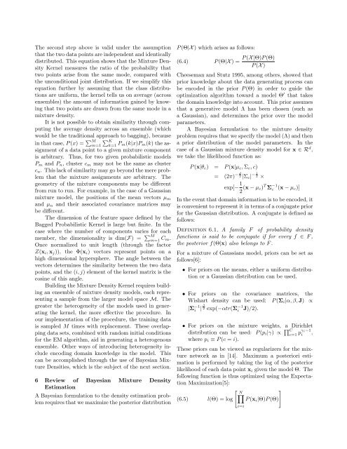
The second step above is valid under the assumptionthat the two data points are independent and identicallydistributed. This equation shows that the Mixture DensityKernel measures the ratio of the probability thattwo points arise from the same mode, compared withthe unconditional joint distribution. If we simplify thisequation further by assuming that the class distributionsare uniform, the kernel tells us on average (acrossensembles) the amount of information gained by knowingthat two points are drawn from the same mode in amixture density.It is not possible to obtain similarity through computingthe average density across an ensemble (whichwould be the traditional approach to bagging), becausein that case, P (x) = ∑ M ∑ Km=1 k=1 P m(k|x)P m (k) the assignmentof a data point to a given mixture componentis arbitrary. Thus, for two given probabilistic modelsP m and P n , cluster c m may not be the same as clusterc n . This lack of similarity may go beyond the mere problemthat the mixture assignments are arbitrary. Thegeometry of the mixture components may be differentfrom run to run. For example, in the case of a Gaussianmixture model, the positions of the mean vectors µ mand µ n and their associated covariance matrices maybe different.The dimension of the feature space defined by theBagged Probabilistic Kernel is large but finite. In thecase where the number of components varies for eachmember, the dimensionality is dim(F) = ∑ Mm=1 C m.Once normalized to unit length (through the factorZ(x i , x j )), the Φ(x i ) vectors represent points on ahigh dimensional hypersphere. The angle between thevectors determines the similarity between the two datapoints, and the (i, j) element of the kernel matrix is thecosine of this angle.Building the Mixture Density Kernel requires buildingan ensemble of mixture density models, each representinga sample from the larger model space M. Thegreater the heterogeneity of the models used in generatingthe kernel, the more effective the procedure. Inour implementation of the procedure, the training datais sampled M times with replacement. These overlappingdata sets, combined with random initial conditionsfor the EM algorithm, aid in generating a heterogenousensemble. Other ways of introducing heterogeneity includeencoding domain knowledge in the model. Thiscan be accomplished through the use of Bayesian MixtureDensities, which is the subject of the next section.6 Review of Bayesian Mixture DensityEstimationA Bayesian formulation to the density estimation problemrequires that we maximize the posterior distributionP (Θ|X ) which arises as follows:(6.4)P (Θ|X ) =P (X |Θ)P (Θ)P (X )Cheeseman and Stutz 1995, among others, showed thatprior knowledge about the data generating process canbe encoded in the prior P (Θ) in order to guide theoptimization algorithm toward a model Θ ′ that takesthe domain knowledge into account. This prior assumesthat a generative model Λ has been chosen (such asa Gaussian), and determines the prior over the modelparameters.A Bayesian formulation to the mixture densityproblem requires that we specify the model (Λ) and thena prior distribution of the model parameters. In thecase of a Gaussian mixture density model for x ∈ R d ,we take the likelihood function as:P (x|θ c ) = P (x|µ c , Σ c , c)= (2π) − d 2 |Σc | − 1 2 ×exp[− 1 2 (x − µ c) T Σ −1c (x − µ c )]In the event that domain information is to be encoded, itis convenient to represent it in terms of a conjugate priorfor the Gaussian distribution. A conjugate is defined asfollows:Definition 6.1. A family F of probability densityfunctions is said to be conjugate if for every f ∈ F ,the posterior f(Θ|x) also belongs to F .For a mixture of Gaussians model, priors can be set asfollows[6]:• For priors on the means, either a uniform distributionor a Gaussian distribution can be used.• For priors on the covariance matrices, theWishart density can be used: P (Σ i |α, β, J) ∝|Σ −1i | β 2 exp(−αtr(Σ −1 J)/2).i• For priors on the mixture weights, a Dirichletdistribution can be used: P (p i |γ) ∝ ∏ Cc=1 pγ i−1i ,where p i ≡ P (c = i).These priors can be viewed as regularizers for the mixturenetwork as in [14]. Maximum a posteriori estimationis performed by taking the log of the posteriorlikelihood of each data point x i given the model Θ. Thefollowing function is thus optimized using the ExpectationMaximization[5]:[ N]∏(6.5) l(Θ) = log P (x i |Θ)P (Θ)i=i
In some cases, details of the underlying distributionare known and can be used to influence the estimateddistribution. For example, in some cases there maybe prior knowledge of the class distribution based onprevious work, in which case the Dirichlet distributionwould be appropriate. Many studies can be performedusing noninformative priors, in which case P (Θ) ≡ 1.In the former case, the mixture density kernel takesdomain information into account, whereas in the lattercase, it is determined directly from the data.7 Comparison with Other KernelsWe now compare the Mixture Density Kernel with threeother types of kernels: the Gaussian or Radial BasisFunction (RBF) kernel and other parametric kernelssuch as the polynomial kernel, the Fisher kernel, andkernel alignment, where the functions are designed tomaximize the accuracy of a prediction.The RBF kernel and other parametric kernel functionsare usually chosen using some heuristic methodwhere the classification accuracy or other criterion isused to choose the best kernel. In the case of the MixtureDensity Kernel, the underlying structure of thedata is used to generate the kernel function. Thus, itcan improve upon the standard set of kernel functionsand can be used in situations where no clear objectivecriterion is available, such as in unsupervised learningproblems like clustering. The parametric kernels are appropriatefor use in unsupervised and supervised problemsalike.The Fisher kernel as developed by Jaakkola andHaussler (1999) [10] and the “Tangent of vectors ofposterior log odds” [17] kernel use probabilistic modelsto generate kernel functions. Kernel Alignment [3]is another method to generate kernel functions, butdoes not use a probabilistic model as its underlyingbasis. However, these kernel functions are optimized fordiscriminative performance and may not be appropriatefor unsupervised problems such as clustering.8 Kernel Clustering in Feature SpaceGirolami, (2001) has given an algorithm to performclustering in the feature space using an approach similarto k-means clustering. A brief review of the methodfollows. The cost function for k-means clustering in thefeature space at a given instant in time is:G Φ = 1 NN∑i=1 k=1[Φ(Z i ) − m Φ k ]K∑q ki [Φ(Z i ) − m Φ k ] T ×where q ki is the cluster membership indicator function(q ki = 1 if vector Z i is a member of cluster k, andzero otherwise), and m Φ kis the cluster center in the featurespace. Thus, if we expand the right-hand side ofthe above equation, and take m Φ k = 1 ∑ NN i=1 q kiΦ(Z i ),which represents the centroid of the cluster in featurespace, we obtain an equation in which only inner productsappear. The nonlinear mapping Φ does not needto be determined explicitly because the kernel functionis taken as the inner product in the feature space:K ij = Φ T (Z i )Φ(Z j ). The objective of kernel clusteringis to find a membership function q and cluster centersm Φ that minimize the cost G Φ . Various methods canbe used to minimize G Φ , including annealing methods(as described in Girolami, 2001) or direct search. Ifthe annealing method is used, the cluster centers areimplicitly defined. However, depending on the kernelfunction used, a direct search approach allows for thepre-image of the cluster center to be explicitly known.Note that K, the number of clusters in the feature space,need not be directly related to ∑ Mc=1 C m, which is thenumber of dimensions of the feature space, nor does Kneed to be a direct function of the number of modesin each mixture ensemble. After the optimization iscompleted, it is possible to compute the uncertainty inthe clustering by computing the entropy of the clusterassignment probability for a given point throughe(x i ) = − ∑ Kk=1 q ki log q ki . We use this quantity tocharacterize the quality of our results in subsequent experiments.9 Experiments and ResultsIn this section, we describe the performance of the MixtureDensity Kernels on a synthetic clustering problemand on a real-world image segmentation problem. Forthe synthetic data set, we show that the algorithm producessuperior results when compared with a standardGaussian kernel.9.1 Clustering with Mixture Density MercerKernels on Synthetic Data Figure 1 shows a plotof the two-dimensional synthetic data. These data aregenerated from a mixture of three Gaussians. Thefirst Gaussian, labelled with the symbol ’o’ has a smallvariance compared with the other two Gaussians. Thesecond Gaussian has a larger spread, and the thirdGaussian partially overlaps the first and second [13].We generated 10,000 points for training, testing, andevaluation of the model. We recognize that this amountof data is very large to specify the model, but wantedto also obtain an estimate of the performance of thealgorithm on a moderate sized data set.The first experiment consists of computing theKernel matrix for the synthetic data using a GaussianKernel as well as the Mixture Density Mercer Kernels.
Page 1 and 2: Mixture Density Mercer Kernels: A M
Page 3: tion yields a symmetric N × N posi
Page 8 and 9: Channel 6 Data0.60.5Channel Spectra
Page 10: References[1] L. Breiman, Bagging p

Mixture Density Mercer Kernels - Intelligent Systems Division - NASA

You also want an ePaper? Increase the reach of your titles

Delete template?

Save as template?