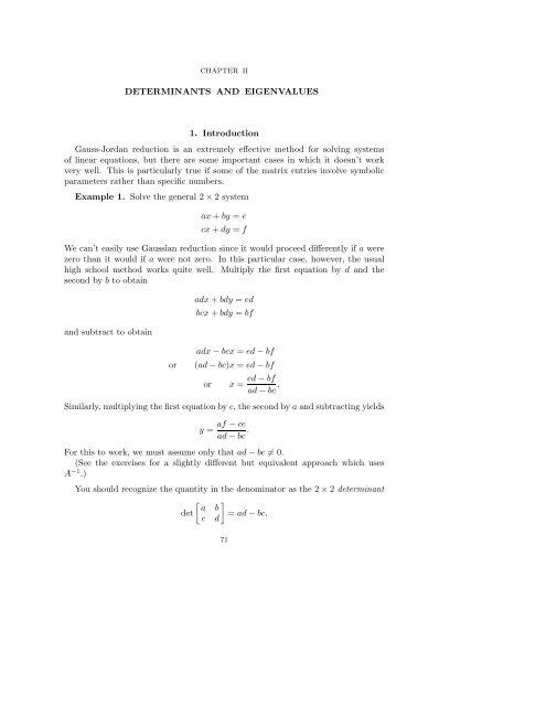
DETERMINANTS AND EIGENVALUES 1. Introduction Gauss ...

74 II. DETERMINANTS AND EIGENVALUES4. Solve the system [ ] [ ]a b x e=c d][y fby multiplying the right hand side by the inverse of the coefficient matrix. Comparewhat you get with the solution obtained in the section.2. Definition of the DeterminantLet A be an n × n matrix. By definitionfor n = 1det [ a ]=a[ ]a11 afor n = 2 det12= aa 21 a 11 a 22 − a 12 a 21 .22As mentioned in the previous section, we can give an explicit formula to definedet A for n = 3 , but an explicit formula for larger n is very difficult to describe.Here is a provisional definition. Form a sum of many terms as follows. Choose anyentry from the first row of A; there are n possible ways to do that. Next, chooseany entry from the second row which is not in the same column as the first entrychosen; there are n − 1 possible ways to do that. Continue in this way until youhave chosen one entry from each row in such a way that no column is repeated;there are n! ways to do that. Now multiply all these entries together to form atypical term. If that were all, it would be complicated enough, but there is onefurther twist. The products are divided into two classes of equal size according toa rather complicated rule and then the sum is formed with the terms in one classmultiplied by +1 and those in the other class multiplied by −1.Here is the definition again for n = 3 arranged to exhibit the signs.⎡det ⎣ a ⎤11 a 12 a 13a 21 a 22 a 23⎦ =a 31 a 32 a 33a 11 a 22 a 33 + a 12 a 23 a 31 + a 13 a 21 a 32− a 11 a 23 a 32 − a 12 a 21 a 33 − a 13 a 22 a 31 .The definition for n = 4 involves 4! = 24 terms, and I won’t bother to write it out.A better way to develop the theory is recursively. That is, we assume thatdeterminants have been defined for all (n − 1) × (n − 1) matrices, and then usethis to define determinants for n × n matrices. Since we have a definition for 1 × 1matrices, this allows us in principle to find the determinant of any n × n matrixby recursively invoking the definition. This is less explicit, but it is easier to workwith.Here is the recursive definition. Let A be an n × n matrix, and let D j (A) be thedeterminant of the (n − 1) × (n − 1) matrix obtained by deleting the jth row andthe first column of A. Then, definedet A = a 11 D 1 (A) − a 21 D 2 (A)+···+(−1) j+1 a j1 D j (A)+···+(−1) n+1 a n1 D n (A).

2. DEFINITION OF THE DETERMINANT 75In words: take each entry in the first column of A, multiply it by the determinantof the (n − 1) × (n − 1) matrix obtained by deleting the first column and that row,and then add up these entries alternating signs as you do.Examples.⎡det ⎣ 2 −1 3⎤1 2 00 3 6⎦ = 2 det[2 03 6]−1 det[ ]−1 3+ 0 det3 6[ ]−1 32 0= 2(12 − 0) − 1(−6 − 9) + 0(...)=24+15=39.Note that we didn’t bother evaluating the 2×2 determinant with coefficient 0. Youshould check that the earlier definition gives the same result.⎡⎤1 2 −1 3⎢ 0 1 2 0⎥det ⎣⎦2 0 3 61 1 2 1⎡= 1 det ⎣ 1 2 0⎤ ⎡0 3 6⎦−0 det ⎣ 2 −1 3⎤0 3 6⎦1 2 11 2 1⎡+ 2 det ⎣ 2 −1 3⎤ ⎡1 2 0⎦−1 det ⎣ 2 −1 3⎤1 2 0⎦.1 2 10 3 6Each of these 3 × 3 determinants may be evaluated recursively. (In fact we just didthe last one in the previous example.) You should work them out for yourself. Theanswers yield⎡⎤1 2 −1 3⎢ 0 1 2 0⎥det ⎣⎦ = 1(3) − 0(...) + 2(5) − 1(39) = −26.2 0 3 61 1 2 1Although this definition allows us to compute the determinant of any n × nmatrix in principle, the number of operations grows very quickly with n. In suchcalculations one usually keeps track only of the multiplications since they are usuallythe most time consuming operations. Here are some values of N(n), the numberof multiplications needed for a recursive calculation of the determinant of an n × ndeterminant. We also tabulate n! for comparison.n N(n) n!2 2 23 6 64 28 245 145 1206 876 720...

76 II. DETERMINANTS AND EIGENVALUESThe recursive method is somewhat more efficient than the formula referred to atthe beginning of the section. For, that formula has n! terms, each of which requiresmultiplying n entries together. Each such product requires n − 1 separate multiplications.Hence, there are (n −1)n! multiplications required altogether. In addition,the rule for determining the sign of the term requires some extensive calculation.However, as the above table indicates, even the number N(n) of multiplicationsrequired for the recursive definition grows faster than n!, so it gets very large veryquickly. Thus, we clearly need a more efficient method to calculate determinants.As is often the case in linear algebra, elementary row operations come to our rescue.Using row operations for calculating determinants is based on the following rulesrelating such operations to determinants.Rule (i): If A ′ is obtained from A by adding a multiple of one row of A to another,then det A ′ = det A.Example 1.⎡det ⎣ 1 2 3⎤2 1 3⎦ = 1(1 − 6) − 2(2 − 6) + 1(6 − 3)=61 2 1⎡det ⎣ 1 2 3⎤0 −3 −3⎦ =1(−3+6)−0(2 − 6) + 1(−6+9)=6.1 2 1Rule (ii): if A ′ is obtained from A by multiplying one row by a scalar c, thendet A ′ = c det A.Example 2.⎡det ⎣ 1 2 0⎤2 4 2⎦ = 1(4 − 2) − 2(2 − 0) + 0(...)=−20 1 1⎡2 det ⎣ 1 2 0⎤1 2 1⎦ = 2(1(2 − 1) − 1(2 − 0) + 0(...)) = 2(−1) = −2.0 1 1One may also state this rule as follows: any common factor of a row of A maybe ‘pulled out’ from its determinant.Rule (iii): If A ′ is obtained from A by interchanging two rows, then det A ′ =− det A.Example 3.det[ ][ ]1 22 1= −3 det =3.2 11 2The verification of these rules is a bit involved, so we relegate it to an appendix,which most of you will want to skip.The rules allow us to compute the determinant of any n × n matrix with specificnumerical entries.

2. DEFINITION OF THE DETERMINANT 77Example 4. We shall calculate the determinant of a 4 × 4 matrix. You shouldmake sure you keep track of which elementary row operations have been performedat each stage.⎡⎤ ⎡⎤ ⎡⎤1 2 −1 1 1 2 −1 1 1 2 −1 1⎢ 0 2 1 2⎥⎢ 0 2 1 2⎥⎢ 0 2 1 2⎥det ⎣⎦ = det ⎣⎦ = det ⎣⎦3 0 1 1 0 −6 4 −2 0 0 7 4−1 6 0 2 0 8 −1 3 0 0 −5 −5⎡⎤ ⎡⎤1 2 −1 11 2 −1 1⎢ 0 2 1 2⎥⎢ 0 2 1 2⎥= −5 det ⎣⎦ = +5 det ⎣⎦0 0 7 40 0 1 10 0 1 10 0 7 4⎡⎤1 2 −1 1⎢ 0 2 1 2⎥= +5 det ⎣⎦.0 0 1 10 0 0 −3We may now use the recursive definition to calculate the last determinant. In eachcase there is only one non-zero entry in the first column.⎡⎤1 2 −1 1 ⎡⎢ 0 2 1 2⎥det ⎣⎦. = 1 det ⎣ 2 1 2⎤0 1 1⎦0 0 1 10 0 −30 0 0 −3[ ]1 1=1·2 det =1·2·1 det [ −3]0 −3=1·2·1·(−3) = −6.Hence, the determinant of the original matrix is 5(−6) = −30.The last calculation is a special case of a general fact which is established inmuch the same way by repeating the recursive definition.⎡⎤a 11 a 12 a 13 ... a 1n0 a 22 a 23 ... a 2ndet0 0 a⎢33 ... a 3n⎣..⎥. ....⎦ = a 11a 22 a 33 ...a nn .0 0 0 ... a nnIn words, the determinant of an upper triangular matrix is the product of its diagonalentries.It is important to be able to tell when the determinant of an n × n matrix Ais zero. Certainly, this will be the case if the first column consists of zeroes, andindeed it turns out that the determinant vanishes if any row or any column consistsonly of zeroes. More generally, if either the set of rows or the set of columns is alinearly dependent set, then the determinant is zero. (That will be the case if therank r

78 II. DETERMINANTS AND EIGENVALUESTheorem 2.1. Let A be an n × n matrix. Then A is singular if and only ifdet A =0. Equivalently, A is invertible, i.e., has rank n, if and only if det A ≠0.Proof. If A is invertible, then Gaussian reduction leads to an upper triangularmatrix with non-zero entries on its diagonal, and the determinant of such a matrixis the product of its diagonal entries, which is also non-zero. No elementary rowoperation can make the determinant zero. For, type (i) operations don’t changethe determinant, type (ii) operations multiply by non-zero scalars, and type (iii)operations change its sign. Hence, det A ≠0.If A is singular, then Gaussian reduction also leads to an upper triangular matrix,but one in which at least the last row consists of zeroes. Hence, at least one diagonalentry is zero, and so is the determinant. □Example 5.⎡det ⎣ 1 1 2⎤2 1 3⎦ = 1(1 − 0) − 2(1 − 0) + 1(3 − 2)=01 0 1so the matrix must be singular. To confirm this, we reduce⎡⎣ 1 1 2⎤ ⎡2 1 3⎦ → ⎣ 1 1 2⎤ ⎡0 −1 −1⎦ → ⎣ 1 1 2⎤0 −1 −1⎦1 0 1 0 −1 −1 0 0 0which shows that the matrix is singular.In the previous section, we encountered 2×2 matrices with symbolic non-numericentries. For such a matrix, Gaussian reduction doesn’t work very well because wedon’t know whether the non-numeric expressions are zero or not.Example 6. Suppose we want to know whether or not the matrix⎡⎤−λ 1 1 1⎢ 1 −λ 0 0⎥⎣⎦1 0 −λ 01 0 0 −λis singular. We could try to calculate its rank, but since we don’t know what λ is,it is not clear how to proceed. Clearly, the row reduction works differently if λ =0than if λ ≠ 0. However, we can calculate the determinant by the recursive method.⎡⎤−λ 1 1 1⎢det ⎣1 −λ 0 0⎥⎦1 0 −λ 01 0 0 −λ⎡=(−λ) det ⎣ −λ 0 0⎤ ⎡0 −λ 0⎦−1 det ⎣ 1 1 1⎤0 −λ 0⎦0 0 −λ0 0 −λ⎡+ 1 det ⎣ 1 1 1⎤ ⎡−λ 0 0⎦−1 det ⎣ 1 1 1⎤−λ 0 0⎦0 0 −λ0 −λ 0=(−λ)(−λ 3 ) − (λ 2 )+(−λ 2 )−(λ 2 )=λ 4 −3λ 2 =λ 2 (λ− √ 3)(λ + √ 3).

80 II. DETERMINANTS AND EIGENVALUESadjacent rows. All told, to switch rows i and j in this way requires 2k + 1 switchesof adjacent rows. The net effect is to multiply the determinant by (−1) 2k+1 = −1as required.There is one important consequence of rule (iii) which we shall use later in theproof of rule (i).Rule (iiie): If an n × n matrix has two equal rows, then det A =0.This is not too hard to see. Interchanging two rows changes the sign of det A,but if the rows are equal, it doesn’t change anything. However, the only numberwith the property that it isn’t changed by changing its sign is the number 0. Hence,det A =0.We next verify rule (ii). Suppose A ′ is obtained from A by multiplying the ithrow by c. Consider the recursive definition(1) det A ′ = a ′ 11D 1 (A ′ )+···+(−1) i+1 a ′ i1D i (A ′ )+···+(−1) n+1 a n1 D n (A).For any j ≠ i, D j (A ′ )=cD j (A) since one of the rows appearing in that determinantis multiplied by c. Also, a ′ j1 = a j1 for j ≠ i. On the other hand, D i (A ′ )=D i (A)since the ith row is deleted in calculating these quantities, and, except for the ithrow, A ′ and A agree. In addition, a ′ i1 = ca i1 so we pick up the extra factor ofc in any case. It follows that every term on the right of (1) has a factor c, sodet A ′ = c det A.Finally, we attack the proof of rule (i). It turns out to be necessary to verify thefollowing stronger rule.Rule (ia): Suppose A, A ′ , and A ′′ are three n × n matrices which agree except inthe ith row. Suppose moreover that the ith row of A is the sum of the ith row of A ′and the ith row of A ′′ . Then det A = det A ′ + det A ′′ .Let’s first see why rule (ia) implies rule (i). We can add c times the jth row ofA to its i row as follows. Let B ′ = A, let B ′′ be the matrix obtained from A byreplacing its ith row by c times its jth row, and let B be the matrix obtained formA by adding c times its jth row to its ith row. Then according to rule (ia), we havedet B = det B ′ + det B ′′ = det A + det B ′′ .On the other hand, by rule (ii), det B ′′ = c det A ′′ where A ′′ has both ith and jthrows equal to the jth row of A. Hence, by rule (iiie), det A ′′ = 0, and det B = det A.Finally, we establish rule (1a). Assume it is known to be true for (n−1)×(n−1)determinants. We have(2) det A = a 11 D 1 (A) −···+(−1) i+1 a i1 D i (A)+···+(−1) n+1 a n1 D n (A).For j ≠ i, the the sum rule (ia) may be applied to the determinants D i (A) becausethe appropriate submatrix has one row which breaks up as a sum as needed. Hence,D j (A) =D j (A ′ )+D j (A ′′ ).

2. DEFINITION OF THE DETERMINANT 81Also, for j ≠ i, we have a j1 = a ′ j1 = a′′ j1 since all the matrices agree in any rowexcept the ith row. Hence, for j ≠ i,a i1 D i (A) =a i1 D i (A ′ )+a i1 D i (A ′′ )=a ′ i1D i (A ′ )+a ′′i1D i (A ′′ ).On the other hand, D i (A) =D i (A ′ )=D i (A ′′ ) because in each case the ith rowwas deleted. But a i1 = a ′ i1 + a′′ i1 ,soa i1 D i (A)=a ′ i1D i (A)+a ′′i1D i (A) =a ′ i1D i (A ′ )+a ′′i1D i (A ′′ ).It follows that every term in (2) breaks up into a sum as required, and det A =det A ′ + det A ′′ .Exercises for Section 2.1. Find the determinants of each of the following matrices. Use whatever methodseems most ⎡ convenient, but seriously consider the use of elementary row operations.(a) ⎣ 1 1 2⎤1 3 5⎦.6 4 1⎡⎤1 2 3 4⎢ 2 1 4 3⎥(b) ⎣⎦.1 4 2 34 3 2 1⎡⎤0 0 0 0 31 0 0 0 2(c) ⎢ 0 1 0 0 1⎥⎣⎦ .0 0 1 0 4⎡0 0 0 1 2(d) ⎣ 0 x y⎤−x 0 z⎦.−y −z 02. Verify the following rules for 2 × 2 determinants.(i) If A ′ is obtained from A by adding a multiple of the first row to the second,then det A ′ = det A.(ii) If A ′ is obtained from A by multiplying its first row by c, then det A ′ =c det A.(iii) If A ′ is obtained from A by interchanging its two rows, then det A ′ = − det A.Rules (i) and (ii) for the first row, together with rule (iii) allow us to derive rules(i) and (ii) for the second row. Explain.3. Derive the following generalization of rule (i) for 2 × 2 determinants.[ ] [ ] [ ]adet′ + a ′′ b ′ + b ′′ a′b= det′ a′′b+ det′′.c dc d c dWhat is the corresponding rule for the second row? Why do you get it for free ifyou use the results of the previous problem?

82 II. DETERMINANTS AND EIGENVALUES4. Find all values of z such that the matrix5. Find all values of λ such that the matrixA =⎡⎣ −λ 1 1 −λ 01⎤⎦0 1 −λis singular.[ ]1 zis singular.z 16. The determinant of the following matrix is zero. Explain why just using therecursive definition of the determinant.⎡⎤2 −2 3 0 44 2 −3 0 1⎢ 6 −5 −2 0 3⎥⎣⎦1 −3 3 0 65 2 12 0 107. If A is n × n, what can you say about det(cA)?8. Suppose A is a non-singular 6 × 6 matrix. Then det(−A) ≠ − det A. Explain.9. Find 2 × 2 matrices A and B such that det(A + B) ≠ det A + det B.10. (a) Show that the number of multiplications N(7) necessary to compute recursivelythe determinant of a 7 × 7 matrix is 6139.(b) (Optional) Find a rule relating N(n) toN(n−1). Use this to write acomputer program to calculate N(n) for any n.3. Some Important Properties of DeterminantsTheorem 2.2 (The Product Rule). Let A and B be n × n matrices. Thendet(AB) = det A det B.We relegate the proof of this theorem to an appendix, but let’s check it in anexampleExample 1. LetA =[ ]2 1, B =1 2[ ]1 −1.1 1Then det A =3,det B = 2, andAB =[ ]3 −13 1

3. SOME IMPORTANT PROPERTIES OF DETERMINANTS 83so det(AB) = 6 as expected.This example has a simple geometric interpretation. Let[ ] [ ]1 −1u = , v = .1 1Then det B is just the area of the parallelogram spanned by the two vectors. Onthe other hand the columns of the product[ ] [3 −1AB =[Au Av] i.e., Au = , Av =3 1]also span a parallelogram which is related to the first parallelogram in a simpleway. One edge is multiplied by a factor 3 and the other edge is fixed. Hence, thearea is multiplied by 3.AuvuAvThus, in this case, in the formuladet(AB) = (det A)(det B)the factor det A tells us how the area of a parallelogram changes if its edges aretransformed by the matrix A. This is a special case of a much more general assertion.The product rule tells us how areas, volumes, and their higher dimensionalanalogues behave when a figure is transformed by a matrix.Transposes. Let A be an m×n matrix. The transpose of A is the n×m matrixfor which the columns are the rows of A. (Also, its rows are the columns of A.) Itis usually denoted A t , but other notations are possible.Examples.⎡[ ]2 0 1A =A t = ⎣ 2 2⎤0 1⎦2 1 21 2⎡A = ⎣ 1 2 3⎤ ⎡0 2 3⎦ A t = ⎣ 1 0 0⎤2 2 0⎦0 0 33 3 3⎡a = ⎣ a ⎤1a 2⎦ a t =[a 1 a 2 a 3 ].a 3

84 II. DETERMINANTS AND EIGENVALUESNote that the transpose of a column vector is a row vector and vice-versa.The following rule follows almost immediately from the definition.Theorem 2.3. Assume A is an m × n matrix and B is an n × p matrix. Then(AB) t = B t A t .Note that the order on the right is reversed.Example 2. Let⎡A = ⎣ 1 2 3⎤ ⎡1 0 2⎦, B = ⎣ 4 0⎤1 1⎦.1 0 02 3ThenwhileB t =⎡ ⎤12 11AB = ⎣ 8 6⎦, so (AB) t =4 0[12 8]411 6 0⎡[ ]4 1 2, A t = ⎣ 1 1 1⎤2 0 0⎦, so B t A t =0 1 33 2 0[12 8]411 6 0as expected.Unless the matrices are square, the shapes won’t even match if the order is notreversed. In the above example A t B t would be a product of a 3 × 3 matrix with a2×3 matrix, and that doesn’t make sense. The example also helps us to understandwhy the formula is true. The i, j-entry of the product is the row by column productof the ith row of A with the jth column of B. However, taking transposes reversesthe roles of rows and columns. The entry is the same, but now it is the product ofthe jth row of B t with the ith column of A t .Theorem 2.4. Let A be an n × n matrix. Thendet A t = det A.See the appendix for a proof, but here is an example.Example 3.⎡det ⎣ 1 0 1⎤2 1 2⎦ = 1(1 − 0) − 2(0 − 0) + 0(...)=10 0 1⎡det ⎣ 1 2 0⎤0 1 0⎦ = 1(1 − 0) − 0(...) + 1(0 − 0)=1.1 2 1The importance of this theorem is that it allows us to go freely from statementsabout determinants involving rows of the matrix to corresponding statements involvingcolumns and vice-versa.Because of this rule, we may use column operations as well as row operationsto calculate determinants. For, performing a column operation is the same astransposing the matrix, performing the corresponding row operation, and thentransposing back. The two transpositions don’t affect the determinant.

3. SOME IMPORTANT PROPERTIES OF DETERMINANTS 85Example.⎡⎤ ⎡⎤1 2 3 0 1 2 2 0⎢ 2 1 3 1⎥⎢ 2 1 1 1⎥det ⎣⎦ = det ⎣⎦3 3 6 2 3 3 3 24 2 6 4 4 2 2 4=0.operation (−1)c1+c3The last step follows because the 2nd and 3rd columns are equal, which implies thatthe rank (dimension of the column space) is less than 4. (You could also subtractthe third column from the second and get a column of zeroes, etc.)Expansion in Minors or Cofactors. There is a generalization of the formulaused for the recursive definition. Namely, for any n × n matrix A, let D ij (A) bethe determinant of the (n − 1) × (n − 1) matrix obtained by deleting the ith rowand jth column of A. Then,(1)det A =n∑(−1) i+j a ij D ij (A)i=1=(−1) 1+j a 1j D 1j (A)+···+(−1) i+j a ij D ij (A)+···+(−1) n+j a nj D nj (A).The special case j = 1 is the recursive definition given in the previous section. Themore general rule is easy to derive from the special case j = 1 by means of columninterchanges. Namely, form a new matrix A ′ by moving the jth column to the firstposition by successively interchanging it with columns j − 1,j−2,...,2,1. Thereare j − 1 interchanges, so the determinant is changed by the factor (−1) j−1 .Nowapply the rule for the first column. The first column of A ′ is the jth column ofA, and deleting it has the same effect as deleting the jth column of A. Hence,a ′ i1 = a ij and D i (A ′ )=D ij (A). Thus,(2)det A =(−1) j−1 det A ′ =(−1) j−1=n ∑i=1(−1) 1+i a ′ i1D i (A ′ )n∑(−1) i+j a ij D ij (A).Similarly, there is a corresponding rule for any row of a matrixdet A =n∑(−1) i+j a ij D ij (A)j=1i=1=(−1) i+1 a i1 D i1 + ···+(−1) i+j a ij D ij (A)+···+(−1) i+n a in D in (A).This formula is obtained from (1) by transposing, applying the corresponding columnrule, and then transposing back.

86 II. DETERMINANTS AND EIGENVALUESExample. Expand the following determinant using its second row.⎡det ⎣ 1 2 3⎤0 6 03 2 1⎦ =(−1) 2+3 0(...)+(−1) 2+2 6 det[1 33 1]+(−1) 2+3 0(...)= 6(1 − 9) = −48.There is some terminology which you may see used in connection with theseformulas. The determinant D ij (A) of the (n − 1) × (n − 1) matrix obtained bydeleting the ith row and jth column is called the i, j-minor of A. The quantity(−1) i+j D ij (A) is called the i, j-cofactor. Formula (1) is called expansion in minors(or cofactors) of the jth column and formula (2) is called expansion in minors (orcofactors) of the ith row. It is not necessary to remember the terminology as longas you remember the formulas and understand how they are used.Cramer’s Rule. One may use determinants to derive a formula for the solutionsof a non-singular system of n equations in n unknowns⎡⎡⎤ ⎤ ⎡ ⎤a 11 a 12 ... a 1n x 1 b 1a⎢ 21 a 22 ... a 2nx⎥ ⎢ 2⎥⎣. . ... .⎦ ⎣.⎦ = b⎢ 2⎣.a n1 a n2 ... a nn x n b nThe formula is called Cramer’s rule, and here it is. For the jth unknown x j , takethe determinant of the matrix formed by replacing the jth column of the coefficientmatrix A by b, and divide it by det A. In symbols,⎥⎦ .⎡⎤a 11 ... b 1 ... a 1nadet ⎢ 21 ... b 2 ... a 2n⎣. ...⎥. ....⎦ax j =n1 ... b n ... a nn⎡a 11 ... a 1j ... a⎤1na 21 ... a 2j ... a 2ndet ⎢⎥⎣⎦. ... . ... .a n1 ... a nj ... a nnExample. ConsiderWe have⎡⎣ 1 0 2⎤⎡1 1 2⎦⎣ x ⎤ ⎡1x 2⎦ = ⎣ 1 ⎤5⎦.2 0 6 x 3 3⎡det ⎣ 1 0 2⎤1 1 2⎦ =2.2 0 6

3. SOME IMPORTANT PROPERTIES OF DETERMINANTS 87(Do you see a quick way to compute that?) Hence,⎡det ⎣ 1 0 2⎤5 1 2⎦3 0 6x 1 == 0 2 2 =0⎡det ⎣ 1 1 2⎤1 5 2⎦2 3 6x 2 == 8 2 2 =4⎡det ⎣ 1 0 1⎤1 1 5⎦2 0 3x 3 == 1 2 2 .You should try to do this by Gauss-Jordan reduction.Cramer’s rule is not too useful for solving specific numerical systems of equations.The only practical method for calculating the needed determinants for n large is touse row (and possibly column) operations. It is usually easier to use row operationsto solve the system without resorting to determinants. However, if the system hasnon-numeric symbolic coefficients, Cramer’s rule is sometimes useful. Also, it isoften valuable as a theoretical tool.Cramer’s rule is related to expansion in minors. You can find further discussionof it and proofs in Section 5.4 and 5.5 of Introduction to Linear Algebra by Johnson,Riess, and Arnold. (See also Section 4.5 of Applied Linear Algebra by Noble andDaniel.)Appendix. Some Proofs. Here are the proofs of two important theoremsstated in this section.The Product Rule. det(AB) = (det A)(det B).Proof. First assume that A is non-singular. Then there is a sequence of rowoperations which reduces A to the identityA → A 1 → A 2 → ...→A k =I.Associated with each of these operations will be a multiplier c i which will dependon the particular operation, anddet A = c 1 det A 1 = c 1 c 2 det A 2 = ···=c 1 c 2 ...c k det A k = c 1 c 2 ...c ksince A k = I and det I = 1. Now apply exactly these row operations to the productABAB → A 1 B → A 2 B → ...→A k B =IB = B.The same multipliers contribute factors at each stage, anddet AB = c 1 det A 1 B = c 1 c 2 det A 2 B = ···=c 1 c 2 ...c} {{ k det B = det A det B.}det A

88 II. DETERMINANTS AND EIGENVALUESAssume instead that A is singular. Then, AB is also singular. (This followsfrom the fact that the rank of AB is at most the rank of A, as mentioned in theExercises for Chapter 1, Section 6. However, here is a direct proof for the record.Choose a sequence of elementary row operations for A, the end result of which isa matrix A ′ with at least one row of zeroes. Applying the same operations to AByields A ′ B which also has to have at least one row of zeroes.) It follows that bothdet AB and det A det B are zero, so they are equal. □The Transpose Rule. det A t = det A.Proof. If A is singular, then A t is also singular and vice-versa. For, the rankmay be characterized as either the dimension of the row space or the dimension ofthe column space, and an n × n matrix is singular if its rank is less than n. Hence,in the singular case, det A =0=detA t .Suppose then that A is non-singular. Then there is a sequence of elementaryrow operationsA → A 1 → A 2 →···→A k =I.Recall from Chapter 1, Section 4 that each elementary row operation may be accomplishedby multiplying by an appropriate elementary matrix. Let C i denote theelementary matrix needed to perform the ith row operation. Then,A → A 1 = C 1 A → A 2 = C 2 C 1 A →···→A k =C k C k−1 ...C 2 C 1 A=I.In other words,A =(C k ...C 2 C 1 ) −1 =C 1 −1 C 2 −1 ...C k −1 .To simplify the notation, let D i = C i −1 . The inverse D of an elementary matrixC is also an elementary matrix; its effect is the row operation which reverses theeffect of C. Hence, we have shown that any non-singular square matrix A may beexpressed as a product of elementary matricesHence, by the product ruleA = D 1 D 2 ...D k .det A = (det D 1 )(det D 2 ) ...(det D k ).On the other hand, we have by rule for the transpose of a productso by the product ruleA t = D k t ...D 2 t D 1 t ,det A t = det(D k t ) ...det(D 2 t ) det(D 1 t ).Suppose we know the rule det D t = det D for any elementary matrix D. Then,det A t = det(D t k ) ...det(D t 2 ) det(D t 1 )= det(D k ) ...det(D 2 ) det(D 1 )= (det D 1 )(det D 2 ) ...(det D k ) = det A.

4. SOME IMPORTANT PROPERTIES OF DETERMINANTS 89(We used the fact that the products on the right are products of scalars and so canbe rearranged any way we like.)It remains to establish the rule for elementary matrices. If D = E ij (c) is obtainedfrom the identity matrix by adding c times its jth row to its ith row, then D t =E ji (c) is a matrix of exactly the same type. In each case, det D = det D t =1.If D = E i (c) is obtained by multiplying the ith row of the identity matrix by c,then D t is exactly the same matrix E i (c). Finally, if D = E ij is obtained from theidentity matrix by interchanging its ith and jth rows, then D t is E ji which in factis just E ij again. Hence, in each case det D t = det D does hold. □Exercises for Section 3.1. Check the validity of the product rule for the product⎡⎣ 1 −2 6⎤⎡2 0 3⎦⎣ 2 3 1⎤1 2 2⎦.−3 1 1 1 1 02. If A and B are n × n matrices, both of rank n, what can you say about therank of AB?3. Find⎡⎤3 0 0 0⎢ 2 2 0 0⎥det ⎣⎦.1 6 4 01 5 4 3Of course, the answer is the product of the diagonal entries. Using the propertiesdiscussed in the section, see how many different ways you can come to thisconclusion.What can you conclude in general about the determinant of a lower triangularsquare matrix?4. (a) Show that if A is an invertible n × n matrix, then det(A −1 )= 1det A . Hint:Let B = A −1 and apply the product rule to AB.(b) Using part(a), show that if A is any n×n matrix and P is an invertible n×nmatrix, then det(PAP −1 ) = det A.5. Why does Cramer’s rule fail if the coefficient matrix A is singular?6. Use Cramer’s rule to solve the system⎡⎤⎡⎤ ⎡ ⎤0 1 0 0 x 1 1⎢ 1 0 1 0⎥⎢x 2 ⎥ ⎢2⎥⎣⎦⎣⎦ = ⎣ ⎦.0 1 0 1 x 3 30 0 1 0 x 4 4Also, solve it by Gauss-Jordan reduction and compare the amount of work you hadto do in each case.

90 II. DETERMINANTS AND EIGENVALUES4. Eigenvalues and Eigenvectors for n × n MatricesOne way in which to understand a matrix A is to examine its effects on thegeometry of vectors in R n . For example, we saw that det A measures the relativechange in area or volume for figures generated by vectors in two or three dimensions.Also, as we have seen in an exercise in Chapter I, Section 2, the multiplesAe 1 ,Ae 2 ,...,Ae n of the standard basis vectors are just the columns of the matrixA. More generally, it is often useful to look at multiples Av for other vectors v.Example 1. LetA =[ ]2 1.1 2Here are some examples of products Av.vAv[ ] [ [ [ [ ]1 1 1 0.5 00 0.5]1]1]1[ ] [ ] [ ] [ [ ]2 2.5 3 2 11 2 3 2.5]2These illustrate a trend for vectors in the first quadrant.Vectors vTransformed vectors AvVectors pointing near one or the other of the two axes are directed closer to thediagonal line. A diagonal vector is transformed into another diagonal vector.Let A be any n × n matrix. In general, if v is a vector in R n , the transformedvector Av will differ from v in both magnitude and direction. However, somevectors v will have the property that Av ends up being parallel to v; i.e., it pointsin the same direction or the opposite direction. These vectors will specify ‘natural’axes for any problem involving the matrix A.

4. EIGENVALUES AND EIGENVECTORS FOR n × n MATRICES 91vvAVPositive eigenvalueAvNegative eigenvalueVectors are parallel when one is a scalar multiple of the other, so we make thefollowing formal definition. A non-zero vector v is called an eigenvector for thesquare matrix A if(1) Av = λvfor an appropriate scalar λ. λ is called the eigenvalue associated with the eigenvectorv.In words, this says that v ≠ 0 is an eigenvector for A if multiplying it by A hasthe same effect as multiplying it by an appropriate scalar. Thus, we may thinkof eigenvectors as being vectors for which matrix multiplication by A takes on aparticularly simple form.It is important to note that while the eigenvector v must be non-zero, the correspondingeigenvalue λ is allowed to be zero.Example 2. LetA =[ ]2 1.1 2We want to see if the system[ ][ ] [ ]2 1 v1 v1=λ1 2 v 2 v 2has non-trivial solutions v 1 ,v 2 . This of course depends on λ. If we write this systemout, it becomesor, collecting terms,In matrix form, this becomes(2)2v 1 + v 2 = λv 1v 1 +2v 2 =λv 2(2 − λ)v 1 + v 2 =0v 1 +(2−λ)v 2 =0.[ ]2 − λ 1v = 0.1 2−λ

92 II. DETERMINANTS AND EIGENVALUESFor any specific λ, this is a homogeneous system of two equations in two unknowns.By the theory developed in the previous sections, we know that it will have nonzerosolutions precisely in the case that the rank is smaller than two. A simplecriterion for that to be the case is that the determinant of the coefficient matrixshould vanish, i.e.,[ ]2 − λ 1det=(2−λ) 2 −1=01 2−λor 4 − 4λ + λ 2 − 1=λ 2 −4λ+3=(λ−3)(λ − 1) = 0.The roots of this equation are λ = 3 and λ = 1. Thus, these and only these scalarsλ can be eigenvalues for appropriate eigenvectors.First consider λ = 3. Putting this in (2) yields(3)[2 − 3 11 2−3]v =Gauss-Jordan reduction yields[ ]−1 1→1 −1[−1 11 −1[ ]1 −1.0 0]v = 0.(As is usual for homogeneous systems, we don’t need to explicitly write downthe augmented matrix, because there are zeroes to the right of the ‘bar’.) Thecorresponding system is v 1 − v 2 = 0, and the general solution is v 1 = v 2 with v 2free. A general solution vector has the form[ ] [ ] [ ]v1 v2 1v = = = vv 2 v 2 .2 1Put v 2 = 1 to obtain[ ]1v 1 =1which will form a basis for the solution space of (3). Any other eigenvector forλ = 3 will be a non-zero multiple of the basis vector v 1 .Consider next the eigenvalue λ = 1. Put this in (2) to obtain(4)[2 − 1 11 2−1]v =[1 11 1]v = 0.In this case, Gauss-Jordan reduction—which we omit—yields the general solutionv 1 = −v 2 with v 2 free. The general solution vector is[ ] [ ]v1 −1v = = vv 2 .2 1Putting v 2 = 1 yields the basic eigenvector[ ]−1v 2 = .1

4. EIGENVALUES AND EIGENVECTORS FOR n × n MATRICES 93The general caseWe redo the above algebra for an arbitrary n × n matrix.eigenvector condition as followsA − λI =⎢⎣Av = λvAv − λv =0Av−λIv =0(A−λI)v =0.First, rewrite theThe last equation is the homogeneous n × n system with n × n coefficient matrix⎡a 11 − λ a 12 ... a 1n⎤a 21 a 22 − λ ... a 2n. . ... .a n1 a n2 ... a nn − λIt has a non-zero solution vector v if and only if the coefficient matrix has rankless than n, i.e., if and only if it is singular. By Theorem 2.1, this will be true ifand only if λ satisfies the characteristic equation⎡⎤a 11 − λ a 12 ... a 1na(5) det(A − λI) = det ⎢ 21 a 22 − λ ... a 2n⎣ .... ... .a n1 a n2 ... a nn − λ⎥⎦ .⎥⎦ =0.As in the example, the strategy for finding eigenvalues and eigenvectors is as follows.First find the roots of the characteristic equation. These are the eigenvalues.Then for each root λ, find a general solution for the system(6) (A − λI)v =0.This gives us all the eigenvectors for that eigenvalue. The solution space of thesystem (6), i.e., the null space of the matrix A − λI, is called the eigenspace correspondingto the eigenvalue λ.Example 3. Consider the matrix⎡A = ⎣ 1 4 3⎤4 1 0⎦.3 0 1The characteristic equation is⎡det(A − λI) = det ⎣ 1 − λ 4 4 1−λ 30⎤⎦3 0 1−λ=(1−λ)((1 − λ) 2 − 0) − 4(4(1 − λ) − 0) + 3(0 − 3(1 − λ)=(1−λ) 3 −25(1 − λ) =(1−λ)((1 − λ) 2 − 25)=(1−λ)(λ 2 − 2λ − 24) = (1 − λ)(λ − 6)(λ +4)=0.

94 II. DETERMINANTS AND EIGENVALUESHence, the eigenvalues are λ =1,λ = 6, and λ = −4. We proceed to find theeigenspaces for each of these eigenvalues, starting with the largest.First, take λ = 6, and put it in (6) to obtain the system⎡⎣ 1 − 6 4 3⎤⎡4 1−6 0 ⎦⎣ v ⎤⎡1v 2⎦ =0 or ⎣ −5 4 3⎤⎡4 −5 0⎦⎣ v ⎤1v 2⎦ =0.3 0 1−6 v 3 3 0 −5 v 3To solve, use Gauss-Jordan reduction⎡⎣ −5 4 3⎤ ⎡⎤ ⎡⎤−1 −1 3 −1 −1 34 −5 0⎦ → ⎣ 4 −5 0⎦ → ⎣ 0 −9 12⎦3 0 −5 3 0 −5 0 −3 4⎡⎤ ⎡⎤−1 −1 3 −1 −1 3→ ⎣ 0 0 0⎦ → ⎣ 0 3 −4⎦0 −3 4 0 0 0⎡→ ⎣ 1 1 −3⎤ ⎡0 1 −4/3⎦ → ⎣ 1 0 −5/3⎤0 1 −4/3⎦.0 0 0 0 0 0Note that the matrix is singular, and the rank is smaller than 3. This must be thecase because the condition det(A − λI) = 0 guarantees it. If the coefficient matrixwere non-singular, you would know that there was a mistake: either the roots ofthe characteristic equation are wrong or the row reduction was not done correctly.The general solution isv 1 =(5/3)v 3v 2 =(4/3)v 3with v 3 free. The general solution vector is⎡v = ⎣ (5/3)v ⎤ ⎡3(4/3)v 3⎦ = v 3⎣ 5/3⎤4/3 ⎦ .v 31Hence, the eigenspace is 1-dimensional. A basis may be obtained by setting v 3 =1as usual, but it is a bit neater to put v 3 = 3 so as to avoid fractions. Thus,⎡v 1 = ⎣ 5 ⎤4 ⎦3constitutes a basis for the eigenspace corresponding to the eigenvalue λ = 6 . Notethat we have now found all eigenvectors for this eigenvalue. They are all the nonzerovectors in this 1-dimensional eigenspace, i.e., all non-zero multiples of v 1 .Next take λ = 1 and put it in (6) to obtain the system⎡⎣ 0 4 3⎤⎡4 0 0⎦⎣ v 1⎦ =0.3 0 0⎤v 2v 3

4. EIGENVALUES AND EIGENVECTORS FOR n × n MATRICES 95Use Gauss-Jordan reduction⎡ ⎤ ⎡ ⎤⎣ 0 4 34 0 0⎦ →···→⎣ 0 1 3/4⎦.3 0 00 0 0The general solution isv 1 =0v 2 =−(3/4)v 3with v 2 free. Thus the general solution vector is⎡ ⎤ ⎡0v = ⎣ −(3/4)v 3⎦ = v 3⎣ 0⎤−3/4 ⎦ .v 31Put v 3 = 4 to obtain a single basis vector⎡v 2 = ⎣ 0⎤−3 ⎦4for the eigenspace corresponding to the eigenvalue λ = 1. The set of eigenvectorsfor this eigenvalue is the set of non-zero multiples of v 2 .Finally, take λ = −4, and put this in (6) to obtain the system⎡⎣ 5 4 3⎤⎡4 5 0⎦⎣ v ⎤1v 2⎦ =0.3 0 5 v 3Solve this by Gauss-Jordan reduction.⎡⎣ 5 4 3⎤ ⎡4 5 0⎦ → ⎣ 1 −1 3⎤ ⎡4 5 0⎦ → ⎣ 1 −1 3⎤0 9 −12 ⎦3 0 5 3 0 5 0 3 −4⎡→ ⎣ 1 −1 3⎤ ⎡0 3 −4⎦ → ⎣ 1 0 5/3⎤0 1 −4/3⎦.0 0 0 0 0 0The general solution isv 1 = −(5/3)v 3v 2 =(4/3)v 3with v 3 free. The general solution vector is⎡v = ⎣ −(5/3)v ⎤ ⎡3(4/3)v 3⎦ = v 3⎣ −5/3⎤4/3 ⎦ .v 3 1

96 II. DETERMINANTS AND EIGENVALUESSetting v 3 = 3 yields the basis vector⎡v 3 = ⎣ −5 ⎤4 ⎦3for the eigenspace corresponding to λ = −4. The set of eigenvectors for this eigenvalueconsists of all non-zero multiples of v 3 .The set {v 1 , v 2 , v 3 } obtained in the previous example is linearly independent.To see this apply Gaussian reduction to the matrix with these vectors as columns:⎡⎣ 5 0 −5⎤ ⎡⎤ ⎡⎤4 −3 43 4 3⎦ → ⎣ 1 0 −10 −3 8⎦ → ⎣ 1 0 −10 1 −8/3⎦.0 4 6 0 0 50/3The reduced matrix has rank 3, so the columns of the original matrix form anindependent set.It is no accident that a set so obtained is linearly independent. The followingtheorem tells us that this will always be the case.Theorem 2.5. Let A be an n × n matrix. Let λ 1 ,λ 2 ,...,λ k be different eigenvaluesof A, and let v 1 , v 2 ,...,v k be corresponding eigenvectors. Then{v 1 , v 2 ,...,v k }is a linearly independent set.See the appendix if you are interested in a proof.Historical Aside. The concepts discussed here were invented by the 19th centuryEnglish mathematicians Cayley and Sylvester, but they used the terms ‘characteristicvector’ and ‘characteristic value’. These were translated into German as‘Eigenvektor’ and ‘Eigenwerte’, and then partially translated back into English—largely by physicists—as ‘eigenvector’ and ‘eigenvalue’. Some English and Americanmathematicians tried to retain the original English terms, but they were overwhelmedby extensive use of the physicists’ language in applications. Nowadayseveryone uses the German terms. The one exception is that we still calldet(A − λI) =0the characteristic equation and not some strange German-English name.Solving Polynomial Equations. To find the eigenvalues of an n × n matrix,you have to solve a polynomial equation. You all know how to solve quadraticequations, but you may be stumped by cubic or higher equations, particularly ifthere are no obvious ways to factor. You should review what you learned in highschool about this subject, but here are a few guidelines to help you.First, it is not generally possible to find a simple solution in closed form foran algebraic equation. For most equations you might encounter in practice, youwould have to use some method to approximate a solution. (Many such methods

4. EIGENVALUES AND EIGENVECTORS FOR n × n MATRICES 97exist. One you may have learned in your calculus course is Newton’s Method.)Unfortunately, an approximate solution of the characteristic equation isn’t muchgood for finding the corresponding eigenvectors. After all, the system(A − λI)v =0must have rank smaller than n for there to be non-zero solutions v. If you replacethe exact value of λ by an approximation, the chances are that the new system willhave rank n. Hence, the textbook method we have described for finding eigenvectorswon’t work. There are in fact many alternative methods for finding eigenvalues andeigenvectors approximately when exact solutions are not available. Whole booksare devoted to such methods. (See Johnson, Riess, and Arnold or Noble and Danielfor some discussion of these matters.)Fortunately, textbook exercises and examination questions almost always involvecharacteristic equations for which exact solutions exist, but it is not always obviouswhat they are. Here is one fact (a consequence of an important result called Gauss’sLemma) which helps us find such exact solutions when they exist. Consider anequation of the formλ n + a 1 λ n−1 + ···+a n−1 λ+a n =0where all the coefficients are integers. (The characteristic equation of a matrixalways has leading coefficient 1 or −1. In the latter case, just imagine you havemultiplied through by −1 to apply the method.) Gauss’s Lemma tells us that if thisequation has any roots which are rational numbers, i.e., quotients of integers, thenany such root is actually an integer, and, moreover, it must divide the constantterm a n . Hence, the first step in solving such an equation should be checking allpossible factors (positive and negative) of the constant term. Once, you know aroot r 1 , you can divide through by λ − r 1 to reduce to a lower degree equation.If you know the method of synthetic division, you will find checking the possibleroots and the polynomial long division much simpler.Example 4. Solveλ 3 − 3λ +2=0.If there are any rational roots, they must be factors of the constant term 2. Hence,we must try 1, −1, 2, −2. Substituting λ = 1 in the equation yields 0, so it is a root.Dividing λ 3 − 3λ +2byλ−1 yieldsλ 3 − 3λ +2=(λ−1)(λ 2 + λ − 2)and this may be factored further to obtainλ 3 − 3λ 2 +2=(λ−1)(λ − 1)(λ +2)=(λ−1) 2 (λ +2).Hence, the roots are λ = 1 which is a double root and λ = −2.Complex Roots. A polynomial equation may end up having complex roots.This can certainly occur for a characteristic equation.

98 II. DETERMINANTS AND EIGENVALUESExample 5. Let[ ]0 −1A = .1 0Its characteristic equation is[ ]−λ −1det(A − λI) = det= λ 2 +1=0.1 −λAs you learned in high school algebra, the roots of this equation are ±i where i isthe imaginary square root of −1.In such a case, we won’t have much luck in finding eigenvectors in R n for such‘eigenvalues’, since solving the appropriate linear equations will yield solutions withnon-real, complex entries. It is possible to develop a complete theory based oncomplex scalars and complex entries, and such a theory is very useful in certainareas like electrical engineering. For the moment, however, we shall restrict ourattention to the theory in which everything is assumed to be real. In that context,we just ignore non-real, complex roots of the characteristic equationAppendix. Proof of the linear independence of sets of eigenvectorsfor distinct eigenvalues. Assume {v 1 , v 2 ,...,v k } is not a linearly independentset, and try to derive a contradiction. In this case, one of the vectors in the setcan be expressed as a linear combination of the others. If we number the elementsappropriately, we may assume that(7) v 1 = c 2 v 2 + ···+c k v r ,where r ≤ k. (Before renumbering, leave out any vector v i on the right if it appearswith coefficient c i = 0.) Note that we may also assume that no vector which appearson the right is a linear combination of the others because otherwise we could expressit so and after combining terms delete it from the sum. Thus we may assume thevectors which appear on the right form a linearly independent set. Multiply (7) onthe left by A. We get(8)Av 1 = c 2 Av 2 + ···+c k Av kλ 1 v 1 =c 2 λ 2 v 2 +...c k λ k v kwhere in (8) we used the fact that each v i is an eigenvector with eigenvalue λ i .Now multiply (7) by λ 1 and subtract from (8). We get(9) 0 = c 2 (λ 2 − λ 1 )v 2 + ···+c k (λ k −λ 1 )v k .Not all the coefficients on the right in this equation are zero. For at least one ofthe c i ≠ 0 (since v 1 ≠ 0), and none of the quantities λ 2 − λ 1 ,...λ k −λ 1 is zero.It follows that (9) may be used to express one of the vectors v 2 ,...,v k as a linearcombination of the others. However, this contradicts the assertion that the set ofvectors appearing on the right is linearly independent. Hence, our initial assumptionthat the set {v 1 , v 2 ,...,v k }is dependent must be false, and the theorem is proved.You should try this argument out on a set {v 1 , v 2 , v 3 } of three eigenvectors tosee if you understand it.

4. EIGENVALUES AND EIGENVECTORS FOR n × n MATRICES 99Exercises for Section 4.1. Find the eigenvalues and eigenvectors for each of the following matrices. Usethe method given in the text for solving the characteristic equation if it has degreegreater[ than two. ]5 −3(a) .2 0⎡⎤3 −2 −2(b) ⎣ 0 0 1⎦.1 0 −1⎡⎤2 −1 −1(c) ⎣ 0 0 −2⎦.0 1 3⎡⎤4 −1 −1(d) ⎣ 0 2 −1⎦.1 0 32. You are a mechanical engineer checking for metal fatigue in a vibrating system.Mathematical ⎡ analysis reduces the problem to finding eigenvectors for the matrixA = ⎣ −2 1 0⎤⎡1 −2 1⎦. A member of your design team tells you that v = ⎣ 1 ⎤1 ⎦ is0 1 −21an eigenvector for A. What is the quickest way for you to check if this is correct?3. As in⎡the previous problem, some other member of your design team tells youthat v = ⎣ 0 ⎤0 ⎦ is a basis for the eigenspace of the same matrix corresponding to0one of its eigenvalues. What do you say in return?4. Under what circumstances can zero be an eigenvalue of the square matrixA? Could A be non-singular in this case? Hint: The characteristic equation isdet(A − λI) =0.5. Let A be a square matrix, and suppose λ is an eigenvalue for A with eigenvectorv. Show that λ 2 is an eigenvalue for A 2 with eigenvector v. What about λ n andA n for n a positive integer?6. Suppose A is non-singular. Show that λ is an eigenvalue of A if and only ifλ −1 is an eigenvalue of A −1 . Hint. Use the same eigenvector.7. (a) Show that det(A−λI) is a quadratic polynomial in λ if A isa2×2 matrix.(b) Show that det(A − λI) is a cubic polynomial in λ if A isa3×3 matrix.(c) What would you guess is the coefficient of λ n in det(A − λI) for A an n × nmatrix?8. (Optional) Let A be an n × n matrix with entries not involving λ. Prove ingeneral that det(A − λI) is a polynomial in λ of degree n. Hint: Assume B(λ) isann×nmatrix such that each column has at most one term involving λ and that term

100 II. DETERMINANTS AND EIGENVALUESis of the form a + bλ. Show by using the recursive definition of the determinantthat det B(λ) is a polynomial in λ of degree at most n. Now use this fact and therecursive definition of the determinant to show that det(A − λI) is a polynomial ofdegree exactly n.9. (Project) The purpose of this project is to illustrate one method for approximatingan eigenvector and the corresponding eigenvalue in cases where exact calculationis not feasible. We use an example in which one can find exact answers bythe usual method, at least if one uses radicals, so we can compare answers to gaugehow effective[ the method is.1 1Let A =1 2Let v 0 =]. Define an infinite sequence of vectors v n in R 2 as follows.[10]. Having defined v n , define v n+1 = Av n . Thus, v 1 = Av 0 , v 2 =Av 1 = A 2 v 0 , v 3 = Av 2 = A 3 v 0 , etc. Then it turns out in this case that asn →∞, the directions of the vectors v n approach the direction of an eigenvectorfor A. Unfortunately, there is one difficulty: the magnitudes |v n | approach [ ] infinity.anTo get get around this problem, proceed as follows. Let v n = and putb nu n = 1 [ ]an /bv n = n. Then the second component is always one, and the firstb n 1[ ]rcomponent r n = a n /b n approaches a limit r and u = is an eigenvector for A.1(a) For the above matrix A, calculate the sequence of vectors v n and and numbersr n n =1,2,3,.... Do the calculations for enough n to see a pattern emerging andso that you can estimate r accurately to 3 decimal places.(b) Once you know an eigenvector u, you can find the corresponding eigenvalueλ by calculating Au. Use your estimate in part (a) to estimate the correspondingλ.(c) Compare this to the roots of the characteristic equation (1−λ)(2−λ)−1 =0.Note that the method employed here only gives you one of the two eigenvalues. Infact, this method, when it works, usually gives the largest eigenvalue.5. DiagonalizationIn many cases, the process outlined in the previous section results in a basis forR n which consists of eigenvectors for the matrix A. Indeed, the set of eigenvectorsso obtained is always linearly independent, so if it is large enough (i.e., has nelements), it will be a basis. When that is the case, the use of that basis toestablish a coordinate system for R n can simplify calculations involving A.Example 1. Let[ ]2 1A = .1 2We found in the previous section that[ ] [ ]1 −1v 1 = , v1 2 =1

5. DIAGONALIZATION 101are eigenvectors respectively with eigenvalues λ 1 = 3 and λ 2 = 1. The set {v 1 , v 2 }is linearly independent, and since it has two elements, it must be a basis for R 2 .Suppose v is any vector in R 2 . We may express it respect to this new basis[ ]y1v = v 1 y 1 + v 2 y 2 =[v 1 v 2 ]y 2where (y 1 ,y 2 ) are the coordinates of v with respect to this new basis. It followsthatAv = A(v 1 y 1 + v 2 y 2 )=(Av 1 )y 1 +(Av 2 )y 2 .However, since they are eigenvectors, each is just multiplied by the correspondingeigenvalue, or in symbolsAv 1 = v 1 (3) and Av 2 = v 2 (1).So(1) A(v 1 y 1 + v 2 y 2 )=v 1 (3y 1 )+v 2 y 2 =[v 1[ ]3y1v 2 ] .y 2In other words, with respect to the new coordinates, the effect of multiplication byA on a vector is to multiply the first new coordinate by the first eigenvalue λ 1 =3and the second new coordinate by the second eigenvalue λ 2 =1.Whenever there is a basis for R n consisting of eigenvectors for A, we say that Ais diagonalizable and that the new basis diagonalizes A.The reason for this terminology may be explained as follows. In the aboveexample, rewrite the left most side of equation (1)[ ]y1A(v 1 y 1 + v 2 y 2 )=A[v 1 v 2 ]y 2and the right most side as[ ]3y1[ v 1 v 2 ] =[vy 1 v 2 ]2[ ][3 0 y10 1y 2].]Since these two are equal, if we drop the common factor on the right, we gety 2[ ]3 0A [ v 1 v 2 ]=[v 1 v 2 ] .0 1Let[ ]1 −1P =[v 1 v 2 ]= ,1 1i.e., P is the 2 × 2 matrix with the basic eigenvectors v 1 , v 2 as columns. Then, theabove equation can be writtenAP = P[ ]3 00 1or P −1 AP =[y1[ ]3 0.0 1

102 II. DETERMINANTS AND EIGENVALUES(The reader should check explicitly in this case that[1 −11 1] −1 [2 11 2][ ]1 −1=1 1[ ] )3 0.0 1By means of these steps, the matrix A has been expressed in terms of a diagonalmatrix with its eigenvalues on the diagonal. This process is called diagonalizationWe shall return in Chapter III to a more extensive discussion of diagonalization.Example 2. Not every n×n matrix A is diagonalizable. That is, it is not alwayspossible to find a basis for R n consisting of eigenvectors for A. For example, letThe characteristic equation isA =[ ]3 1.0 3[ ]3 − λ 1det=(3−λ) 2 =0.0 3−λThere is only one root λ = 3 which is a double root of the equation. To find thecorresponding eigenvectors, we solve the homogeneous system (A − 3I)v = 0. Thecoefficient matrix [ ]3 − 3 1=0 3−3[ ]0 10 0is already reduced, and the corresponding system has the general solutionThe general solution vector isv =v 2 =0, v 1 free.[ ] [ ]v1 1= v0 1 = v0 1 e 1 .Hence, the eigenspace for λ = 3 is one dimensional with basis {e 1 }. There are noother eigenvectors except for multiples of e 1 . Thus, we can’t possibly find a basisfor R 2 consisting of eigenvectors for A.Note how Example 2 differs from the examples which preceded it; its characteristicequation has a repeated root. In fact, we have the following general principle.If the roots of the characteristic equation of a matrix are all distinct, then thereis necessarily a basis for R n consisting of eigenvectors, and the matrix is diagonalizable.In general, if the characteristic equation has repeated roots, then the matrixneed not be diagonalizable. However, we might be lucky, and such a matrix maystill be diagonalizable.

5. DIAGONALIZATION 103Example 3. Consider the matrix⎡A = ⎣ 1 1 −1⎤−1 3 −1⎦.−1 1 1First solve the characteristic equationdet⎡⎣ 1 − λ −1 1 3−λ −1−1⎤⎦ =−1 1 1−λ(1 − λ)((3 − λ)(1 − λ)+1)+(1−λ+1)−(−1+3−λ)=(1−λ)(3 − 4λ + λ 2 +1)+2−λ−2+λ=(1−λ)(λ 2 − 4λ +4)=(1−λ)(λ − 2) 2 =0.Note that 2 is a repeated root. We find the eigenvectors for each of these eigenvalues.For λ = 2 we need to solve (A − 2I)v =0.⎡⎤ ⎡−1 1 −1⎣−1 1 −1⎦ → ⎣ 1 −1 1⎤0 0 0⎦.−1 1 −1 0 0 0The general solution of the system is v 1 = v 2 − v 3 with v 2 ,v 3 free. The generalsolution vector for that system is⎡ ⎤ ⎤ ⎤v =⎣ v 2 − v 3v 2v 3⎦ = v 2⎡⎣ 1 10⎦ + v 3⎡⎣ −1 0 ⎦ .1The eigenspace is two dimensional. Thus, for the eigenvalue λ = 2 we obtain twobasic eigenvectors⎡ ⎤ ⎡ ⎤v 1 = ⎣ 1 1 ⎦ , v 2 = ⎣ −1 0 ⎦ ,01and any eigenvector for λ = 2 is a non-trivial linear combination of these.For λ = 1, we need to solve (A − I)v =0.⎡⎤ ⎡⎤ ⎡ ⎤⎣ 0 1 −1⎣ 1 −1 0⎣ 1 0 −1−1 2 −1−1 1 0⎦ →0 1 −10 0 0⎦ →0 1 −10 0 0The general solution of the system is v 1 = v 3 ,v 2 = v 3 with v 3 free. The generalsolution vector is⎡v = ⎣ v ⎤ ⎡3v 3⎦ = v 3⎣ 1 ⎤1 ⎦ .v 3 1⎦.

104 II. DETERMINANTS AND EIGENVALUESThe eigenspace is one dimensional, and a basic eigenvector for λ =1is⎡v 3 = ⎣ 1 ⎤1⎦.1It is not hard to check that the set of these basic eigenvectors⎧ ⎡⎨⎩ v 1 = ⎣ 1 ⎤ ⎡1 ⎦ , v 2 = ⎣ −1 ⎤ ⎡0 ⎦ , v 3 = ⎣ 1 ⎤⎫⎬1 ⎦⎭01 1is linearly independent, so it is a basis for R 3 .The matrix is diagonalizable.In the above example, the reason we ended up with a basis for R 3 consistingof eigenvectors for A was that there were two basic eigenvectors for the doubleroot λ = 2. In other words, the dimension of the eigenspace was the same as themultiplicity.Theorem 2.6. Let A be an n × n matrix. The dimension of the eigenspacecorresponding to a given eigenvalue is always less than or equal to the multiplicityof that eigenvalue. In particular, if all the roots of the characteristic polynomialare real, then the matrix will be diagonalizable provided, for every eigenvalue, thedimension of the eigenspace is the same as the multiplicity of the eigenvalue. If thisfails for at least one eigenvalue, then the matrix won’t be diagonalizable.Note. If the characteristic polynomial has non-real, complex roots, the matrixalso won’t be diagonalizable in our sense, since we require all scalars to be real.However, it might still be diagonalizable in the more general theory allowing complexscalars as entries of vectors and matrices.Exercises for Section 5.1. (a) Find a basis for R 2 consisting of eigenvectors for[ ]1 2A = .2 1(b) Let P be the matrix with columns the basis vectors you found in part (a).Check that P −1 AP is diagonal with the eigenvalues on the diagonal.2. (a) Find a basis for R 3 consisting of eigenvectors for⎡A = ⎣ 1 2 −4⎤2 −2 −2⎦.−4 −2 1(b) Let P be the matrix with columns the basis vectors in part (a). CalculateP −1 AP and check that it is diagonal with the diagonal entries the eigenvalues youfound.

6. THE EXPONENTIAL OF A MATRIX 1053. (a) Find the eigenvalues and eigenvectors for⎡A = ⎣ 2 1 1⎤0 2 1⎦.0 0 1(b) Is A diagonalizable?4. (a) Find a basis for R 3 consisting of eigenvectors for⎡A = ⎣ 2 1 1⎤1 2 1⎦.1 1 2(b) Find a matrix P such that P −1 AP is diagonal. Hint: See Problem 1.5. Suppose A is a 5 × 5 matrix with exactly three (real) eigenvalues λ 1 ,λ 2 ,λ 3 .Suppose these have multiplicities m 1 ,m 2 , and m 3 as roots of the characteristicequation. Let d 1 ,d 2 , and d 3 respectively be the dimensions of the eigenspaces forλ 1 ,λ 2 , and λ 3 . In each of the following cases, are the given numbers possible, andif so, is A diagonalizable?(a) m 1 =1,d 1 =1,m 2 =2,d 2 =2,m 3 =2,d 3 =2.(b) m 1 =2,d 1 =1,m 2 =1,d 2 =1,m 3 =2,d 3 =2.(c) m 1 =1,d 1 =2,m 2 =2,d 2 =2,m 3 =2,d 3 =2.(d) m 1 =1,d 1 =1,m 2 =1,d 2 =1,m 3 =1,d 3 =1.6. Tell if each of the following matrices is diagonalizable or not.[ ] [ ] [ ]5 −2 1 1 0 −1(a), (b)(c)−2 8 0 1 1 06. The Exponential of a MatrixRecall the series expansion for the exponential functione x =1+x+ x22! + x33! + ···= ∞∑This series is specially well behaved. It converges for all possible x.There are situations in which one would like to make sense of expressions of theform f(A) where f(x) is a well defined function of a scalar variable and A is asquare matrix. One way to do this is to try to make a series expansion. We showhow to do this for the exponential function.Definee A = I + A + 1 2 A2 + 1 ∞∑ A n3! A3 + ···=n! .A little explanation is necessary. Each term on the right is an n × n matrix. Ifthere were only a finite number of such terms, there would be no problem, and thesum would also be an n × n matrix. In general, however, there are infinitely manyterms, and we have to worry about whether it makes sense to add them up.n=0n=0x nn! .

106 II. DETERMINANTS AND EIGENVALUESThenExample 1. LetHence,A = t[ ]0 1.−1 0[ ]A 2 = t 2 −1 00 −1[ ]A 3 = t 3 0 −11 0[ ]A 4 = t 4 1 00 1[ ]A 5 = t 5 0 1−1 0.[ ] [ ]e A 1 0 0 1= +t + 1 [ ]−1 00 1 −1 0 2 t2 + 1 [ ]0 −10 −1 3! t3 +...1 0[ 1−t 2=2 + t4t34!− ... t−3! + t55! − ... ]−t+ t33! − t55! + ... 1− t2 2 + t4[ ]4! − ...cos t sin t=.− sin t cos tAs in the example, a series of n × n matrices yields a separate series for eachof the n 2 possible entries. We shall say that such a series of matrices converges ifthe series it yields for each entry converges. With this rule, it is possible to showthat the series defining e A converges for any n × n matrix A, but the proof is abit involved. Fortunately, it is often the case that we can avoid worrying aboutconvergence by appropriate trickery. In what follows we shall generally ignore suchmatters and act as if the series were finite sums.The exponential function for matrices obeys the usual rules you expect an exponentialfunction to have, but sometimes you have to be careful.(1) If 0 denotes the n × n zero matrix, then e 0 = I.(2) The law of exponents holds if the matrices commute, i.e., if B and C aren × n matrices such that BC = CB, then e B+C = e B e C .(3) If A is an n × n constant matrix, then d dt eAt = Ae At = e At A. (It is worthwriting this in both orders because products of matrices don’t automaticallycommute.)Here are the proofs of these facts.(1) e 0 = I +0+ 1 2 02 +···=I.

6. THE EXPONENTIAL OF A MATRIX 107(2) See the Exercises.(3) Here we act as if the sum were finite (although the argument would work ingeneral if we knew enough about convergence of series of matrices.)ddt eAt = d (I + tA + 1 dt2 t2 A 2 + 1 3! t3 A 3 + ···+ 1 )j! tj A j +...=0+A+ 1 2 (2t)A2 + 1 3! (3t2 )A 3 + ···+ 1 j! (jtj−1 )A j + ...=A+tA 2 + 1 2 t2 A 3 1+ ···+(j−1)! tj−1 A j + ...=A(I +tA + 1 2 t2 A 2 1+ ···+(j−1)! tj−1 A j−1 + ...)=Ae At .Note that in the next to last step A could just as well have been factored out onthe right, so it doesn’t matter which side you put it on.Exercises for Section 6.[ ]λ 01. (a) Let A = . Show that0 µe At =[ ]eλt00 e µt .⎡⎤λ 1 0 ... 00 λ(b) Let A = ⎢ 2 ... 0⎣.⎥. ....⎦ . Such a matrix is called a diagonal matrix.0 0 ... λ nWhat can you say about e At ?[ ]0 02. (a) Let N = . Calculate e1 0Nt .⎡(b) Let N = ⎣ 0 0 0⎤1 0 0⎦. Calculate e Nt .0 1 0⎡⎤0 0 ... 0 01 0 ... 0 0(c) Let N be an n × n matrix of the form0 1 ... 0 0⎢⎥⎣. . ... . .⎦ . What is the0 0 ... 1 0smallest integer k satisfying N k = 0? What can you say about e Nt ?[ ]λ 03. (a) Let A = . Calculate e1 λAt . Hint: use A = λI +(A−λI). Note thatA and N = A − λI commute.

108 II. DETERMINANTS AND EIGENVALUES⎡(b) Let A = ⎣ λ 0 0⎤1 λ 0⎦. Calculate e At .0 1 λ⎡⎤λ 0 ... 0 01 λ ... 0 0(c) Let A be an n × n matrix of the form0 1 ... 0 0⎢⎥⎣. . ... . .⎦ . What can you0 0 ... 1 λsay about e At = e λt e (A−λI)t ?4. Let A be an n × n matrix, and let P be a non-singular n × n matrix. ShowthatPe At P −1 = e PAP−1t .5. Let B and C be two n × n matrices such that BC = CB. Prove thate B+C = e B e C .Hint: You may assume that the binomial theorem applies to commuting matrices,i.e.,(B + C) n = ∑ n!i!j! Bi C j .6. LetB =(a) Show that BC ≠ CB.(b) Show thate B =[ ]0 10 0[ ]1 10 1i+j=nC =e C =[ ]0 0.−1 0[ ]1 0.−1 1(c) Show that e B e C ≠ e B+C . Hint: B + C = J, where e tJ was calculated in thetext.7. ReviewExercises for Section 7.⎡1. What is det ⎣ 0 0 1⎤0 2 1⎦? Find the answer without using the recursive formula3 2 1or Gaussian reduction.2. Tell whether each of the following statements is true or false. and, if false,explain why.(a) If A and B are n × n matrices then det(AB) = det A det B.(b) If A is an n × n matrix and c is a scalar, then det(cA) =cdet A.(c) If A is m × n and B is n × p, then (AB) t = B t A t .(d) If A is invertible, then so it A t .

7. REVIEW 109⎡3. A = ⎣ 0 1 1⎤1 0 1⎦. Find the eigenvalues and eigenvectors of A.1 1 0⎡⎤1 3 1 1⎢ 1 2 4 3⎥4. Find det ⎣⎦.2 4 1 11 1 6 15. Each of the following statements is not generally true. In each case explainbriefly why it is false.(a) An n × n matrix A is invertible if and only if det A =0.(b) If A is an n × n real matrix, then there is a basis for R n consisting ofeigenvectors for A.(c) det A t = det A. Hint. Are these defined?⎡6. Let A = ⎣ 2 1 6⎤ ⎡1 3 1⎦.Isv=⎣ 1 ⎤1⎦an eigenvector for A? Justify your answer.2 2 517. (a) The characteristic equation of⎡A = ⎣ 2 −4 1⎤0 3 0⎦1 −4 2is −(λ − 3) 2 (λ⎡− 1)=0. IsAdiagonalizable? Explain.(b) Is B = ⎣ 1 2 3⎤0 4 5⎦ diagonalizable? Explain.0 0 68. Let A be an n × n matrix with the property that the sum of all the entries ineach row is always the same number a. Without using determinants, show that thecommon sum a is an eigenvalue. Hint: What is the corresponding eigenvector?

110 II. DETERMINANTS AND EIGENVALUES