DETERMINANTS AND EIGENVALUES 1. Introduction Gauss ...

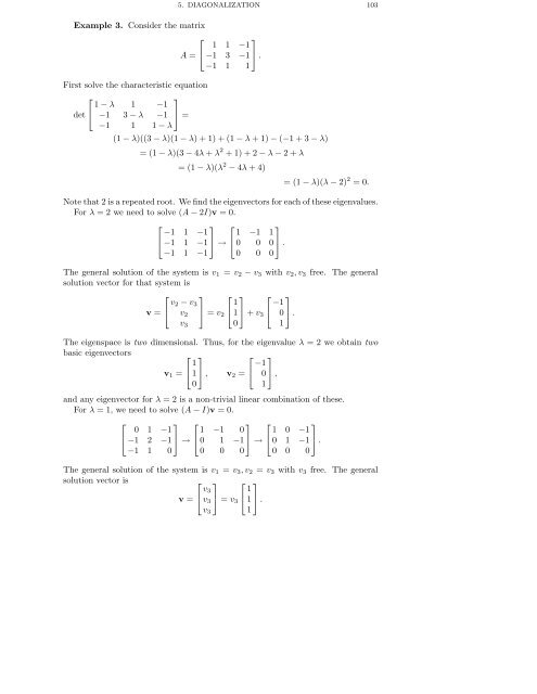
5. DIAGONALIZATION 103Example 3. Consider the matrix⎡A = ⎣ 1 1 −1⎤−1 3 −1⎦.−1 1 1First solve the characteristic equationdet⎡⎣ 1 − λ −1 1 3−λ −1−1⎤⎦ =−1 1 1−λ(1 − λ)((3 − λ)(1 − λ)+1)+(1−λ+1)−(−1+3−λ)=(1−λ)(3 − 4λ + λ 2 +1)+2−λ−2+λ=(1−λ)(λ 2 − 4λ +4)=(1−λ)(λ − 2) 2 =0.Note that 2 is a repeated root. We find the eigenvectors for each of these eigenvalues.For λ = 2 we need to solve (A − 2I)v =0.⎡⎤ ⎡−1 1 −1⎣−1 1 −1⎦ → ⎣ 1 −1 1⎤0 0 0⎦.−1 1 −1 0 0 0The general solution of the system is v 1 = v 2 − v 3 with v 2 ,v 3 free. The generalsolution vector for that system is⎡ ⎤ ⎤ ⎤v =⎣ v 2 − v 3v 2v 3⎦ = v 2⎡⎣ 1 10⎦ + v 3⎡⎣ −1 0 ⎦ .1The eigenspace is two dimensional. Thus, for the eigenvalue λ = 2 we obtain twobasic eigenvectors⎡ ⎤ ⎡ ⎤v 1 = ⎣ 1 1 ⎦ , v 2 = ⎣ −1 0 ⎦ ,01and any eigenvector for λ = 2 is a non-trivial linear combination of these.For λ = 1, we need to solve (A − I)v =0.⎡⎤ ⎡⎤ ⎡ ⎤⎣ 0 1 −1⎣ 1 −1 0⎣ 1 0 −1−1 2 −1−1 1 0⎦ →0 1 −10 0 0⎦ →0 1 −10 0 0The general solution of the system is v 1 = v 3 ,v 2 = v 3 with v 3 free. The generalsolution vector is⎡v = ⎣ v ⎤ ⎡3v 3⎦ = v 3⎣ 1 ⎤1 ⎦ .v 3 1⎦.