DETERMINANTS AND EIGENVALUES 1. Introduction Gauss ...

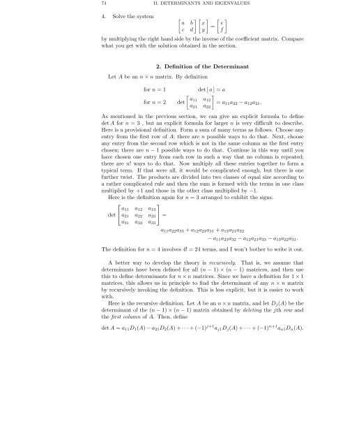
74 II. DETERMINANTS AND EIGENVALUES4. Solve the system [ ] [ ]a b x e=c d][y fby multiplying the right hand side by the inverse of the coefficient matrix. Comparewhat you get with the solution obtained in the section.2. Definition of the DeterminantLet A be an n × n matrix. By definitionfor n = 1det [ a ]=a[ ]a11 afor n = 2 det12= aa 21 a 11 a 22 − a 12 a 21 .22As mentioned in the previous section, we can give an explicit formula to definedet A for n = 3 , but an explicit formula for larger n is very difficult to describe.Here is a provisional definition. Form a sum of many terms as follows. Choose anyentry from the first row of A; there are n possible ways to do that. Next, chooseany entry from the second row which is not in the same column as the first entrychosen; there are n − 1 possible ways to do that. Continue in this way until youhave chosen one entry from each row in such a way that no column is repeated;there are n! ways to do that. Now multiply all these entries together to form atypical term. If that were all, it would be complicated enough, but there is onefurther twist. The products are divided into two classes of equal size according toa rather complicated rule and then the sum is formed with the terms in one classmultiplied by +1 and those in the other class multiplied by −1.Here is the definition again for n = 3 arranged to exhibit the signs.⎡det ⎣ a ⎤11 a 12 a 13a 21 a 22 a 23⎦ =a 31 a 32 a 33a 11 a 22 a 33 + a 12 a 23 a 31 + a 13 a 21 a 32− a 11 a 23 a 32 − a 12 a 21 a 33 − a 13 a 22 a 31 .The definition for n = 4 involves 4! = 24 terms, and I won’t bother to write it out.A better way to develop the theory is recursively. That is, we assume thatdeterminants have been defined for all (n − 1) × (n − 1) matrices, and then usethis to define determinants for n × n matrices. Since we have a definition for 1 × 1matrices, this allows us in principle to find the determinant of any n × n matrixby recursively invoking the definition. This is less explicit, but it is easier to workwith.Here is the recursive definition. Let A be an n × n matrix, and let D j (A) be thedeterminant of the (n − 1) × (n − 1) matrix obtained by deleting the jth row andthe first column of A. Then, definedet A = a 11 D 1 (A) − a 21 D 2 (A)+···+(−1) j+1 a j1 D j (A)+···+(−1) n+1 a n1 D n (A).