Ding Wang 2012 Neurocomputing

More documents

Recommendations

Info

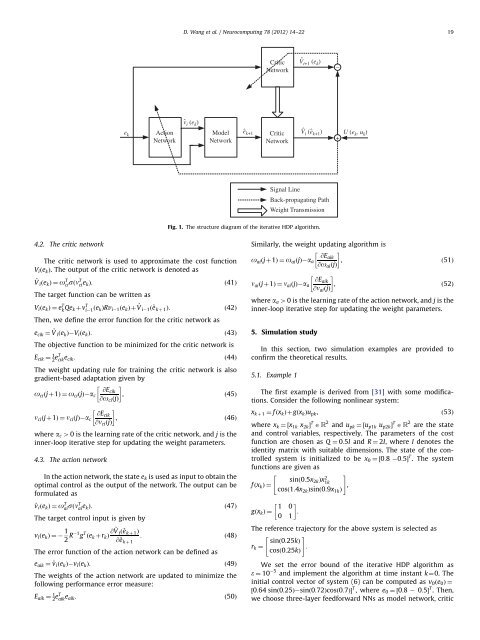
D. Wang et al. / Neurocomputing 78 (2012) 14–22 19CriticNetworkVî+1 (e k )_e kActionNetworkvî (e k )ModelNetworkeˆk+1 Critic Vî (eˆk+1 ) U (e k , u k )Network+Signal LineBack-propagating PathWeight TransmissionFig. 1. The structure diagram of the iterative HDP algorithm.4.2. The critic networkThe critic network is used to approximate the cost functionV i ðe k Þ. The output of the critic network is denoted as^V i ðe k Þ¼o T cisðn T ci e kÞ:ð41ÞThe target function can be written asV i ðe k Þ¼e T k Qe k þv T i 1 ðe kÞRv i 1 ðe k Þþ ^V i 1 ðê k þ 1 Þ: ð42ÞThen, we define the error function for the critic network ase cik ¼ ^V i ðe k Þ V i ðe k Þ: ð43ÞThe objective function to be minimized for the critic network isE cik ¼ 1 2 eT cik e cik:ð44ÞThe weight updating rule for training the critic network is alsogradient-based adaptation given by @Eo ci ðjþ1Þ¼o ci ðjÞ a cikc , ð45Þ@o ci ðjÞ @En ci ðjþ1Þ¼n ci ðjÞ a cikc , ð46Þ@n ci ðjÞwhere a c 40 is the learning rate of the critic network, and j is theinner-loop iterative step for updating the weight parameters.4.3. The action networkIn the action network, the state e k is used as input to obtain theoptimal control as the output of the network. The output can beformulated as^v i ðe k Þ¼o T aisðn T ai e kÞ:ð47ÞThe target control input is given byv i ðe k Þ¼1 2 R 1 g T ðe k þr k Þ @ ^V i ðê k þ 1 Þ: ð48Þ@ê k þ 1The error function of the action network can be defined ase aik ¼ ^v i ðe k Þ v i ðe k Þ: ð49ÞThe weights of the action network are updated to minimize thefollowing performance error measure:E aik ¼ 1 2 eT aik e aik:ð50ÞSimilarly, the weight updating algorithm is @Eo ai ðjþ1Þ¼o ai ðjÞ a aika , ð51Þ@o ai ðjÞ @En ai ðjþ1Þ¼n ai ðjÞ a aika , ð52Þ@n ai ðjÞwhere a a 40 is the learning rate of the action network, and j is theinner-loop iterative step for updating the weight parameters.5. Simulation studyIn this section, two simulation examples are provided toconfirm the theoretical results.5.1. Example 1The first example is derived from [31] with some modifications.Consider the following nonlinear system:x k þ 1 ¼ f ðx k Þþgðx k Þu pk ,ð53Þwhere x k ¼½x 1k x 2k Š T AR 2 and u pk ¼½u p1k u p2k Š T AR 2 are the stateand control variables, respectively. The parameters of the costfunction are chosen as Q ¼ 0:5I and R ¼ 2I, where I denotes theidentity matrix with suitable dimensions. The state of the controlledsystem is initialized to be x 0 ¼½0:8 0:5Š T . The systemfunctions are given as" #sinð0:5x 2k Þx 2 1kf ðx k Þ¼,cosð1:4x 2k Þsinð0:9x 1k Þgðx k Þ¼ 1 0 :0 1The reference trajectory for the above system is selected as"r k ¼sinð0:25kÞ#:cosð0:25kÞWe set the error bound of the iterative HDP algorithm ase ¼ 10 5 and implement the algorithm at time instant k¼0. Theinitial control vector of system (6) can be computed as v 0 ðe 0 Þ¼½0:64 sinð0:25Þ sinð0:72Þcosð0:7ÞŠ T , where e 0 ¼½0:8 0:5Š T . Then,we choose three-layer feedforward NNs as model network, critic
20D. Wang et al. / Neurocomputing 78 (2012) 14–22network and action network with the structures 4–8–2, 2–8–1,2–8–2, respectively. The initial weights of the three networks areall set to be random in ½ 1; 1Š. It should be mentioned that themodel network should be trained first. We train the modelnetwork for 1000 steps using 500 data samples under the learningrate a m ¼ 0:1. After the training of the model network is completed,the weights are kept unchanged. Then, we train the criticnetwork and the action network for 20 iterations (i.e., fori ¼ 1; 2, ...,20) with each iteration of 2000 training steps to makesure the given error bound e ¼ 10 5 is reached. In the trainingprocess, the learning rate a c ¼ a a ¼ 0:05. The convergence processof the cost function of the iterative HDP algorithm is shown inFig. 2, for k¼0. We can see that the iterative cost functionsequence does converge to the optimal cost function quiterapidly, which indicates the effectiveness of the iterative HDPalgorithm. Therefore, we have 9V 19 ðe 0 Þ V 20 ðe 0 Þ9re, which meansthat the number of steps of the e-optimal control is K e ðe 0 Þ¼19.Besides, the e-optimal control law m n e ðe 0Þ for system (6) can alsobe obtained during the iteration process.Next, we compute the near-optimal tracking control law fororiginal system (1) using (35) and apply it to the controlled systemfor 40 time steps. The obtained state curves are shown inThe state trajectory and the reference trajectory21.510.50−0.5−10 5 10 15 20 25 30 35 40Time stepsFig. 4. The state trajectory x 2 and the reference trajectory r 2 .r 2x 22.11.5u p1The cost function21.91.81.71.61.51.40 5 10 15 20Iteration stepsFig. 2. The convergence process of the cost function.The tracking control trajectories10.50−0.5−1−1.50 5 10 15 20 25 30 35 40Time stepsFig. 5. The tracking control trajectories u p .u p2The state trajectory and the reference trajectory1.510.50−0.5−10 5 10 15 20 25 30 35 40Time stepsFig. 3. The state trajectory x 1 and the reference trajectory r 1 .r 1x 1The tracking error10.50−0.5−1−1.50 5 10 15 20 25 30 35 40Time stepsFig. 6. The tracking error e.e 1e 2
Page 4 and 5: D. Wang et al. / Neurocomputing 78
Page 8 and 9: D. Wang et al. / Neurocomputing 78

Ding Wang 2012 Neurocomputing

Create successful ePaper yourself

Delete template?

Save as template?