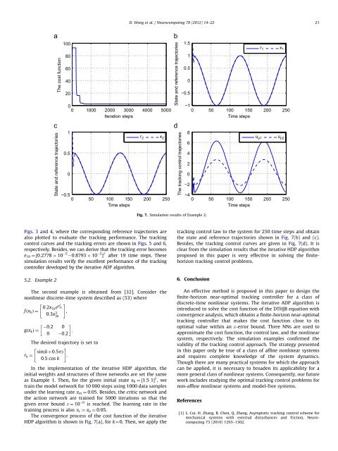
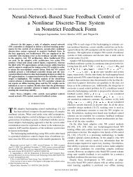
D. <strong>Wang</strong> et al. / <strong>Neurocomputing</strong> 78 (<strong>2012</strong>) 14–22 21The cost function1008060402000 1000 2000 3000 4000 5000Iteration stepsState and reference trajectories1.510.50−0.5r 1 x 1−10 50 100 150 200 250Time stepsState and reference trajectories10.50−0.50 50 100 150 200 250Time stepsr 2 x 28u p1 u p26The tracking control trajectories−2Fig. 7. Simulation results of Example 2.420−40 50 100 150 200 250Time stepsFigs. 3 and 4, where the corresponding reference trajectories arealso plotted to evaluate the tracking performance. The trackingcontrol curves and the tracking errors are shown in Figs. 5 and 6,respectively. Besides, we can derive that the tracking error becomese 19 ¼½0:2778 10 5 20:8793 10 5 Š T after 19 time steps. Thesesimulation results verify the excellent performance of the trackingcontroller developed by the iterative ADP algorithm.5.2. Example 2The second example is obtained from [32]. Consider thenonlinear discrete-time system described as (53) where"f ðx k Þ¼0:2x #1ke x2 2k0:3x 3 ,2k0:2 0gðx k Þ¼:0 0:2The desired trajectory is set to"r k ¼sinðkþ0:5pÞ#:0:5 cos kIn the implementation of the iterative HDP algorithm, theinitial weights and structures of three networks are set the sameas Example 1. Then, for the given initial state x 0 ¼½1:5 1Š T ,wetrain the model network for 10 000 steps using 1000 data samplesunder the learning rate a m ¼ 0:05. Besides, the critic network andthe action network are trained for 5000 iterations so that thegiven error bound e ¼ 10 6 is reached. The learning rate in thetraining process is also a c ¼ a a ¼ 0:05.The convergence process of the cost function of the iterativeHDP algorithm is shown in Fig. 7(a), for k¼0. Then, we apply thetracking control law to the system for 250 time steps and obtainthe state and reference trajectories shown in Fig. 7(b) and (c).Besides, the tracking control curves are given in Fig. 7(d). It isclear from the simulation results that the iterative HDP algorithmproposed in this paper is very effective in solving the finitehorizontracking control problems.6. ConclusionAn effective method is proposed in this paper to design thefinite-horizon near-optimal tracking controller for a class ofdiscrete-time nonlinear systems. The iterative ADP algorithm isintroduced to solve the cost function of the DTHJB equation withconvergence analysis, which obtains a finite-horizon near-optimaltracking controller that makes the cost function close to itsoptimal value within an e-error bound. Three NNs are used toapproximate the cost function, the control law, and the nonlinearsystem, respectively. The simulation examples confirmed thevalidity of the tracking control approach. The strategy presentedin this paper only be true of a class of affine nonlinear systemsand requires complete knowledge of the system dynamics.Though there are many practical systems for which the approachcan be applied, it is necessary to broaden its applicability for amore general class of nonlinear systems. Consequently, our futurework includes studying the optimal tracking control problems fornon-affine nonlinear systems and model-free systems.References[1] L. Cui, H. Zhang, B. Chen, Q. Zhang, Asymptotic tracking control scheme formechanical systems with external disturbances and friction, <strong>Neurocomputing</strong>73 (2010) 1293–1302.
22D. <strong>Wang</strong> et al. / <strong>Neurocomputing</strong> 78 (<strong>2012</strong>) 14–22[2] S. Devasia, D. Chen, B. Paden, Nonlinear inversion-based output tracking,IEEE Trans. Autom. Control 41 (1996) 930–942.[3] G. Tang, Y. Liu, Y. Zhang, Approximate optimal output tracking control fornonlinear discrete-time systems, Control Theory Appl. 27 (2010) 400–405.[4] F.L. Lewis, V.L. Syrmos, Optimal Control, Wiley, New York, 1995.[5] R.E. Bellman, Dynamic Programming, Princeton University Press, Princeton,NJ, 1957.[6] T. Poggio, F. Girosi, Networks for approximation and learning, Proc. IEEE78 (1990) 1481–1497.[7] S. Jagannathan, Neural Network Control of Nonlinear Discrete-time Systems,CRC Press, Boca Raton, FL, 2006.[8] W. Yu, Recent Advances in Intelligent Control Systems, Springer-Verlag,London, 2009.[9] P.J. Werbos, Approximate dynamic programming for real-time control andneural modeling, in: White, D.A., Sofge, D.A. (Eds.), Handbook of IntelligentControl, Van Nostrand Reinhold, New York, 1992 (Chapter 13).[10] P.J. Werbos, Intelligence in the brain: a theory of how it works and how tobuild it, Neural Networks 22 (2009) 200–212.[11] P.J. Werbos, Advanced forecasting methods for global crisis warning andmodels of intelligence, General Syst. Yearb. 22 (1977) 25–38.[12] J.J. Murray, C.J. Cox, G.G. Lendaris, R. Saeks, Adaptive dynamic programming,IEEE Trans. Syst. Man Cybern. Part C Appl. Rev. 32 (2002) 140–153.[13] F.Y. <strong>Wang</strong>, H. Zhang, D. Liu, Adaptive dynamic programming: an introduction,IEEE Comput. Intell. Mag. 4 (2009) 39–47.[14] F.L. Lewis, D. Vrabie, Reinforcement learning and adaptive dynamic programmingfor feedback control, IEEE Circuits Syst. Mag. 9 (2009) 32–50.[15] J. Si, A.G. Barto, W.B. Powell, D.C. Wunsch (Eds.), Handbook of Learning andApproximate Dynamic Programming, IEEE Press, Wiley, New York, 2004.[16] A. Al-Tamimi, F.L. Lewis, M. Abu-Khalaf, Discrete-time nonlinear HJB solutionusing approximate dynamic programming: convergence proof, IEEE Trans.Syst. Man Cybern. Part B Cybern. 38 (2008) 943–949.[17] D.P. Bertsekas, J.N. Tsitsiklis, Neuro-Dynamic Programming, Athena Scientific,Belmont, MA, 1996.[18] J. Si, Y.T. <strong>Wang</strong>, On-line learning control by association and reinforcement,IEEE Trans. Neural Networks 12 (2001) 264–276.[19] D.V. Prokhorov, D.C. Wunsch, Adaptive critic designs, IEEE Trans. NeuralNetworks 8 (1997) 997–1007.[20] R.S. Sutton, A.G. Barto, Reinforcement Learning: An Introduction, The MITPress, Cambridge, MA, 1998.[21] D. Liu, X. Xiong, Y. Zhang, Action-dependent adaptive critic designs,in: Proceedings of International Joint Conference on Neural Networks,Washington, DC, July 2001, pp. 990–995.[22] D. Liu, Y. Zhang, H. Zhang, A self-learning call admission control scheme forCDMA cellular networks, IEEE Trans. Neural Networks 16 (2005) 1219–1228.[23] F.Y. <strong>Wang</strong>, N. Jin, D. Liu, Q. Wei, Adaptive dynamic programming for finitehorizonoptimal control of discrete-time nonlinear systems with e-errorbound, IEEE Trans. Neural Networks 22 (2011) 24–36.[24] S.N. Balakrishnan, V. Biega, Adaptive-critic based neural networks for aircraftoptimal control, J. Guidance Control Dyn. 19 (1996) 893–898.[25] S.N. Balakrishnan, J. <strong>Ding</strong>, F.L. Lewis, Issues on stability of ADP feedbackcontrollers for dynamic systems, IEEE Trans. Syst. Man Cybern. Part B Cybern.38 (2008) 913–917.[26] G.K. Venayagamoorthy, R.G. Harley, D.C. Wunsch, Comparison of heuristicdynamic programming and dual heuristic programming adaptive critics forneurocontrol of a turbogenerator, IEEE Trans. Neural Networks 13 (2002)764–773.[27] G.K. Venayagamoorthy, R.G. Harley, D.C. Wunsch, Implementation of adaptivecritic-based neurocontrollers for turbogenerators in a multimachinepower system, IEEE Trans. Neural Networks 14 (2003) 1047–1064.[28] M. Abu-Khalaf, F.L. Lewis, Nearly optimal control laws for nonlinear systemswith saturating actuators using a neural network HJB approach, Automatica41 (2005) 779–791.[29] T. Cheng, F.L. Lewis, M. Abu-Khalaf, A neural network solution for fixed-finaltime optimal control of nonlinear systems, Automatica 43 (2007) 482–490.[30] H. Zhang, Y. Luo, D. Liu, Neural-network-based near-optimal control for aclass of discrete-time affine nonlinear systems with control constraints,IEEE Trans. Neural Networks 20 (2009) 1490–1503.[31] T. Dierks, S. Jagannathan, Optimal tracking control of affine nonlineardiscrete-time systems with unknown internal dynamics, in: Proceedings ofJoint 48th IEEE Conference on Decision and Control and 28th Chinese ControlConference, Shanghai, PR China, December 2009, pp. 6750–6755.[32] H. Zhang, Q. Wei, Y. Luo, A novel infinite-time optimal tracking controlscheme for a class of discrete-time nonlinear systems via the greedy HDPiteration algorithm, IEEE Trans. Syst. Man Cybern. Part B Cybern. 38 (2008)937–942.[33] D. Vrabie, O. Pastravanu, M. Abu-Khalaf, F.L. Lewis, Adaptive optimal controlfor continuous-time linear systems based on policy iteration, Automatica45 (2009) 477–484.[34] K.G. Vamvoudakis, F.L. Lewis, Online actor-critic algorithm to solve thecontinuous-time infinite horizon optimal control problem, Automatica46 (2010) 878–888.[35] R. Song, H. Zhang, Y. Luo, Q. Wei, Optimal control laws for time-delaysystems with saturating actuators based on heuristic dynamic programming,<strong>Neurocomputing</strong> 73 (2010) 3020–3027.[36] Y.M. Park, M.S. Choi, K.Y. Lee, An optimal tracking neuro-controller fornonlinear dynamic systems, IEEE Trans. Neural Networks 7 (1996)1099–1110.<strong>Ding</strong> <strong>Wang</strong> received the B.S. degree in mathematicsfrom Zhengzhou University of Light Industry, Zhengzhou,China, and the M.S. degree in operational researchand cybernetics from Northeastern University, Shenyang,China, in 2007 and 2009, respectively. He iscurrently working toward the Ph.D. degree in the KeyLaboratory of Complex Systems and IntelligenceScience, Institute of Automation, Chinese Academy ofSciences, Beijing, China. His research interests includeadaptive dynamic programming, neural networks, andintelligent control.Derong Liu received the Ph.D. degree in electricalengineering from the University of Notre Dame, NotreDame, IN, in 1994. Dr. Liu was a Staff Fellow withGeneral Motors Research and Development Center,Warren, MI, from 1993 to 1995. He was an AssistantProfessor in the Department of Electrical and ComputerEngineering, Stevens Institute of Technology, Hoboken,NJ, from 1995 to 1999. He joined the University ofIllinois at Chicago in 1999, where he became a FullProfessor of Electrical and Computer Engineering and ofComputer Science in 2006. He was selected for the ‘‘100Talents Program’’ by the Chinese Academy of Sciencesin 2008. Dr. Liu was an Associate Editor of the IEEETransactions on Circuits and Systems—Part I: Fundamental Theory and Applications(1997–1999), the IEEE Transactions on Signal Processing (2001–2003), the IEEETransactions on Neural Networks (2004–2009), the IEEE Computational IntelligenceMagazine (2006–2009), and the IEEE Circuits and Systems Magazine (2008–2009),and the Letters Editor of the IEEE Transactions on Neural Networks (2006–2008).Currently, he is the Editor-in-Chief of the IEEE Transactions on Neural Networks andan Associate Editor of the IEEE Transactions on Control Systems Technology. Hereceived the Michael J. Birck Fellowship from the University of Notre Dame (1990),the Harvey N. Davis Distinguished Teaching Award from Stevens Institute ofTechnology (1997), the Faculty Early Career Development (CAREER) Award fromthe National Science Foundation (1999), the University Scholar Award fromUniversity of Illinois (2006), and the Overseas Outstanding Young Scholar Awardfrom the National Natural Science Foundation of China (2008).Qinglai Wei received the B.S. degree in automation, theM.S. degree in control theory and control engineering, andthe Ph.D. degree in control theory and control engineering,from the Northeastern University, Shenyang, China, in2002, 2005, and 2008, respectively. He is currently apostdoctoral fellow with the Key Laboratory of ComplexSystems and Intelligence Science, Institute of Automation,Chinese Academy of Sciences, Beijing, China. His researchinterests include neural-networks-based control, nonlinearcontrol, adaptive dynamic programming, and theirindustrial applications.