A new correlation for predicting hydrate formation conditions for ...

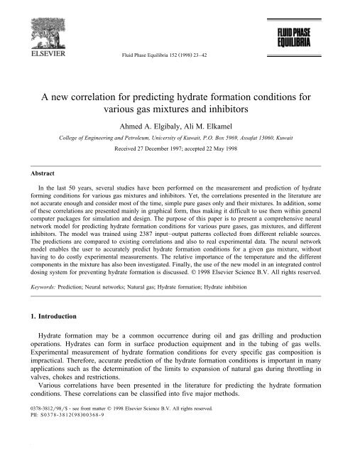
24( )A.A. Elgibaly, A.M. ElkamelrFluid Phase Equilibria 152 1998 23–42The first is the K-value method, which utilizes the vapor–solid equilibrium constants for predictinghydrate-forming conditions wx 1 . The method is based on the concept that hydrates are solid solutions.The hydrate forming conditions are predicted from empirically estimated vapor–solid equilibriumconstants given byK vs,isyirx iŽ 1.where yiis the mole fraction of the ith hydrocarbon component in the gas phase considered on awater-free basis and xiis the mole fraction of the same component in the solid phase on a water-freebasis. The hydrate formation conditions should satisfynÝ iis1y rK s1 Ž 2.vs,iInclusion of non-hydrocarbon gases such as CO 2, N2 and H 2S may cause inaccurate results. Mann etal. wx 2 presented new K-charts that cover a wide range of pressures and temperatures. These charts canbe an alternate to the tentative charts constructed by Carson and Katz wx 1 , which are not a function ofstructure or composition. The new charts are based on the statistical thermodynamic calculations.The second method is the gas–gravity plot developed by Katz wx 3 . The plot relates the hydrateformation pressure and temperature with gas gravity defined as the apparent molecular weight of a gasmixture divided by that of air. This method is a simple graphical technique that may be useful for aninitial estimate of hydrate formation conditions. The hydrate formation chart was generated from alimited amount of experimental data and a more substantial amount of calculations based on theK-value method. A statistical accuracy analysis reported by Sloan wx 4 , showed that this method is notaccurate. For the same gas gravity, different mixtures may lead to about 50% error in the predictedpressure. Over the last 50 years, enormous experimental data on hydrate formation conditions havebeen collected and hence a more accurate gas gravity chart can be developed. One purpose of thisstudy is to develop such chart as will be explained later.The third method consists of empirical correlations developed according to the following form byHolder et al. wx 5 and Makogon wx 6 for selected pure gases.PsexpŽ aqbrT . Ž 3.where a and b are empirical coefficients that depend on the temperature range for each gas. Fornatural gas, another correlation was presented following a general equation based on the gas gravityby Makogon wx 6 .ln Ps2.3026bq0.1144Ž TqkT 2 . Ž 4.where bs2.681–3.811 gq1.679 g 2 and ksy0.006q0.011 gq0.011 g 2 .Based on the fit to Katz wx 3 gas–gravity plot, Kobayashi et al. wx 7 developed the followingempirical equation for hydrate-forming conditions of natural gases.Ž . Ž . Ž . Ž .2 231 2 g 3Ž . 4 g 5 g Ž . 6Ž . 7 gTs1r A qA ln g qA ln P qA ln g qA ln g ln P qA ln P qA ln gŽ . Ž . Ž . Ž .2 2 34 38 g 9 g 10 11 g 12 gqA ln g Ž ln P . qA ln g Ž ln P . qA Ž ln P . qA ln g qA ln g Ž ln P .Ž . Ž .2 2 3 413 g 14 g 15qA ln g Ž ln P . qA ln g Ž ln P . qA Ž ln P . Ž 5.

26( )A.A. Elgibaly, A.M. ElkamelrFluid Phase Equilibria 152 1998 23–42published in the research literature. The predictions of the neural network models are compared to theavailable correlations and also to experimental data. The remainder of this paper will first give a briefoverview of artificial neural networks and then presents the design, training, testing and validation ofthe various neural network models discussed previously. The testing and validation of the modelsindicate that the use of neural networks is promising for the accurate prediction of hydrate formationconditions for generalized gas systems. This apparent success leads us to discuss the integration ofsuch models with inhibitor dosing devices for accurate hydrate prevention and to minimize the cost ofinhibitors used.2. Artificial neural networksNeural networks are so named because they mimic the behavior of biological neurons and learn bytrial and error. Neural networks are first subjected to a set of training data consisting of input datatogether with corresponding outputs. After a sufficient number of training iterations, the neuralnetwork learns the patterns in the data fed to it and creates an internal model, which it uses to makepredictions for new inputs.The foundation of an artificial neural network is the neuron or processing element Ž PE. Ž Fig. 1 ..Each processing element i receives an input vector I Ž I swI , I ,..., I x.i i i1 i2 in which is weighted witha weight vector W ŽWswW , W ,..., W x.i i i1 i2 in . The processing element then calculates an output O i,usually by using a sigmoidal function, which is a monatomic, continuously differentiable function,i.e.,1Oisf Ž Ii. s Ž 6.1qexpŽ yI .iThe PEs are arranged in a special topology or architecture. There are several possible architecturesthat can be used, however the most commonly used one is the multi-layer back-propagationFig. 1. A typical neuron i in the hidden layer.

( )A.A. Elgibaly, A.M. ElkamelrFluid Phase Equilibria 152 1998 23–42 27architecture Ž Fig. 2 .. This type of network contains a layer of input neurons, a layer of output neurons,and one or several hidden layers of intermediate neurons. All the neurons are connected with differentweights. In addition, there is a bias neuron that is connected to each neuron in the hidden and outputlayers. The input layer receives input from the outside world and processes them and transmits themto the hidden layer. The output from a neuron in the hidden and the output layers is also given by Eq.Ž 6 .. In this case, the input I to a neuron in these layers is calculated from:ž Ý /iI s W O qW O Ž 7.i ij j iB Bjwhere the sum over j represents all neurons in the previous layer and OBis an invariant output fromthe bias neuron. The weight Wijrepresents the connection weight between neurons i and j and theweight WiBis the connection weight between neuron i and the bias neuron.The back-propagation neural network is applicable to a wide variety of problems and is thepredominant supervised training algorithm. The term ‘back-propagation’ indicates the method bywhich the network is trained, and the term ‘supervised learning’ implies that the network is trainedthrough a set of available input–output patterns. The network is repeatedly exposed to theseinput–output relationships and the weights among the neurons are continuously adjusted until thenetwork ‘learns’ the correct input–output behavior. Initially, all the weights are set randomly and thedifference or error between the desired and calculated outputs is calculated. This error is propagatedback through the network and is used to update the weights among neurons iteratively. This updateFig. 2. A one hidden layer feed forward neural network.

( )A.A. Elgibaly, A.M. ElkamelrFluid Phase Equilibria 152 1998 23–42 29Finally in model-D, the hydrocarbon-non-hydrate-formers such as i-pentane, n-pentane Žlumped aspentane ., and hexane plus; and the inhibitors including methanol, sodium chloride, ethylene glycol,calcium chloride, and ethanol are collectively included to the previous model, i.e.,Psf T, y , y , y , y , y , y , y , y , y , y q , y , y , y , y , y Ž 11.Ž .4 C1 C2 C3 i-C4 n-C4 CO2 N H2S C5 C6 MeOH EG EtOH NaCl CaCl2In order to achieve appropriate computation stability during the learning phase of ANN, the domainof input variation should be within the range of the used data. This was performed by the followingscaling rule:ToldyTold,minTnews Ž 12.T yTold,maxold,minwhere T and T are the maximum and minimum input values of previous Ž or initial.old,max old,minvariable, whereas Toldand Tneware the scaled values of old and new variables, respectively. Theoutput variable was transformed by using the logarithmic rule w27 x, i.e.,PnewslnŽ P . Ž 13.2.1. Data usedThe hydrate phase–equilibrium data used in this study were mainly obtained from the comprehenw22x. The author provided a magnificent overview of the experimental datasive book by Sloanavailable in the literature from 1934 to 1990. Additional data were also collected from other sourcesw18–21,23,28–30 x. A total of 2389 data entries have been examined. The data were divided intosingle, binary, ternary, and multi-component systems Ž Table 1 .. The experimental data on purehydrocarbon components include methane, ethane, propane, i-butane, and pentane Žlumped i-pentaneand n-pentane .. Heavier components including crude oil constituents are lumped in hexane plus.Because of the lack of success in forming hydrates of pure n-butane, no reliable data were reported inthe literature for this component. Even the role of n-butane in multi-component hydrocarbon systemswas not obvious w31 x. However, the data available for gas mixtures containing n-butane wereconsidered. The pure non-hydrocarbon components involve carbon dioxide, nitrogen, and hydrogensulfide. The consistency of the data was examined by Sloan w22xand assessed in the present study forthe new data.The phase equilibrium data for binary, ternary, and mixtures of these components were investigated.Depending on the pressure and temperature of the system, the data represented one or more ofTable 1Types of the gases and materials used in the correlationsTypeHydrocarbon hydrate-formersNon-hydrocarbon hydrate-formersHydrocarbon non-hydrate-formersComponentC , C , C , i-C , n-C1 2 3 4 4CO , N, H S2 2qi-C , n-C , C5 5 6Inhibitors MeOH, EG, EtOH, NaCl, CaCl 2

( )A.A. Elgibaly, A.M. ElkamelrFluid Phase Equilibria 152 1998 23–42 31Table 3Properties and statistical parameters of the neural network modelsModel No. of input No. of data No. of No. of hidden AAPE SSEvariables entries neurons layersANN-A 2 1012 25 1 32.657 0.9770ANN-B 9 1012 50 1 40.265 0.9521ANN-C 11 1791 40 1 20.860 0.9864ANN-D 16 2389 40 1 19.416 0.9794Katz wx 3 correlation presented in the year 1945. In order to compare with Katz wx 3 gravity charts, themodel was trained by data for the pure hydrate-formers: C 1, C 2, C 3, i-C 4, and n-C 4, and theirmixtures. Using 1012 input data entries, a correlation for ANN model-A was obtained with onehidden layer and 25 neurons. As illustrated in Table 3, the model correlated the experimental datawith an average error of 32.657% and sum-squares error Ž SSE.of 0.977.ANN gravity model-A was used to prepare an analogous chart to that of Katz wx 3 . Fig. 3 shows thehydrate formation conditions for various gas gravities: 0.554, 0.6, 0.7, 0.8, 0.9, and 1.0. While thefirst three curves are monotonically decreasing with gravity over a wide range of temperaturevariation, the latter three curves Ž gG0.8.show a limited range of temperature due to the lack of data.For gas gravities greater than 1.0, the corresponding curves Ž not shown on the graph for simplicity .,become closer and ambiguous. This ambiguity can be attributed in part to the lack of data over thatwide range of temperature shown in Fig. 3 and to the fact that using gravity only is not enough todefine the corresponding thermodynamic system.Fig. 3. Gas gravity chart by ANN model-A.

32( )A.A. Elgibaly, A.M. ElkamelrFluid Phase Equilibria 152 1998 23–42Fig. 4. Predictions by ANN gravity model-A and other correlations for 0.554 gas gravity.Fig. 4 illustrates the hydrate formation pressures for an example gas gravity of 0.554. Results arepresented as measured and calculated by ANN model-A and other methods including Holder et al. wx 5 ,Makogon wx 6 , Katz wx 3 , and Kobayashi et al. wx 7 . The latter three methods were chosen because theyare mainly based on gravity graphical plots. As shown in Fig. 4, while the methods of Holder et al.Fig. 5. Cross plot of ANN model-A.

( )A.A. Elgibaly, A.M. ElkamelrFluid Phase Equilibria 152 1998 23–42 33wx wx wx wx5 , Katz 3 and Kobayashi et al. 7 are accurate over a limited data range, the Makogon 6correlation gave the least accuracy for the examined data. The ANN model-A provided reasonablyaccurate results over a wide range of hydrate formation conditions.The cross plot shown in Fig. 5, compares the measured hydrate formation pressure with thatpredicted by ANN model-A. The data are presented for various phase equilibria of pure hydrocarboncomponents and their mixtures. As can be seen, relatively little scatter is obtained around the 458-line.This indicates a good agreement between the measured and calculated results.3.2. ANN compositional modelsIn the next phase of this study, three ANN models were developed to consider the relationshipsindicated in Eq. Ž 9. through Eq. Ž 11 .. Several neural network architectures were attempted to find outthe best accuracy. A one-hidden layer network was found to be suitable. The number of neurons inthe hidden layer was varied until a minimum sum squared error was obtained. Table 3 demonstratesthe final neural network properties and statistical parameters of these models. The number of neuronstabulated for the different models delivered acceptable results. They were justified by the correspondingcross plot verifications Ž Figs. 6–8 ..The ANN model-B was developed to include the composition of the hydrocarbon hydrate-formersas indicated in Eq. Ž 11 .. The model showed lower average error and sum-squares error than those ofthe ANN model-A. This may be due to the lack of data for pure n-butane, though data on its mixturewith other components were available w31 x. The model is capable to predict the hydrate formationpressure, which fitted well the experimental pressure for the methane–ethane system at differentproportions as shown in Fig. 9.Fig. 6. Prediction of hydrate formation conditions by ANN model-B for methane–ethane mixture.

34( )A.A. Elgibaly, A.M. ElkamelrFluid Phase Equilibria 152 1998 23–42Fig. 7. Cross plot of ANN model-B.3.3. Comparison of deÕeloped compositional ANN modelsANN model-D is the most comprehensive of the compositional models considered. The accuracyŽ .of this model is checked against the other more specialized models Models-B and -C . These latterFig. 8. Cross plot of ANN model-C.

( )A.A. Elgibaly, A.M. ElkamelrFluid Phase Equilibria 152 1998 23–42 35Fig. 9. Cross plot of ANN model-D.models were considered to facilitate comparisons with models available in the literature and also tocheck whether or not more specialized models might lead to better accuracies than a generalizedmodel. Table 3 compares the statistical parameters for these models. The results show that thecomprehensive ANN model-D deliver a competitive correlation coefficient. For a total number of dataentries of 2387, this model gives an average absolute error of 19.4% and sum-squares error of 0.9794.The cross plot of this model Ž Fig. 9.confirms this fact.To further check the accuracy of the generalized model-D compared to models-C and -D, a smallsubset of the data was considered. In Table 4 the experimental hydrate-forming pressure is tabulatedagainst the pressure predicted by different compositional models for this data subset. The resultsreveal that the ANN model-D fit is good and compares well with the other models. Therefore, it canbe concluded that the comprehensive ANN model-D can be generally used to predict the hydrateformation pressure for all system compositions. The predictions of the statistical thermodynamicmodel Ž STM.are also included in Table 4 for comparison purposes.The new model can predict the hydrate formation conditions for gas systems existing in one ormore of the following phase regions: I–H–V, L w–H–L hc, L w–H–L hc–V, and L w–H–L hc on thegeneral equilibrium pressure–temperature plot. Contrary to the statistical thermodynamic model, thedeveloped model does not necessarily require a priori knowledge of the number and type of phasesbefore prediction.3.4. Validation of the deÕeloped modelsThe validation of the new models was examined by using data that have not been considered intheir developments. Random samples of extra measured data points, which represent different phases

36( )A.A. Elgibaly, A.M. ElkamelrFluid Phase Equilibria 152 1998 23–42Table 4Calculations of hydrate formation pressure for methane–ethane system by various compositional modelsTemp. Ž K. Composition Ž mol% . Pressure Ž kPa.Methane Ethane Measured STM ANN model-B ANN model-C ANN model-DPredicted APE Predicted APE Predicted APE Predicted APE284 1.60 98.4 1810 1716 5.19 1810 0.131 1720 4.89 1720 5.13286 1.60 98.4 2310 2249 2.64 2300 0.227 2360 2.36 2190 5.21288 1.60 98.4 3080 3026 1.75 3400 10.4 3790 23.1 3240 5.12279 4.70 95.3 990 924 6.67 1420 43.6 855 13.6 1180 19.0283 4.70 95.3 1710 1508 11.81 1750 2.40 1490 13.2 1660 3.07288 4.70 95.3 2990 2951 1.30 2560 14.3 3340 11.8 2520 15.6282 17.7 82.3 1420 1385 2.46 1340 5.48 1350 4.68 1780 25.6285 17.7 82.3 2140 1983 7.34 2200 2.73 2190 21.8 1840 14.2287 17.7 82.3 3000 2545 15.17 8902 3.69 2990 0.339 3180 6.00275 56.4 43.6 945 893 5.50 893 5.48 1290 36.4 946 0.0958278 56.4 43.6 1290 1233 4.42 1360 5.69 1410 910 1290 0.0237283 56.4 43.6 2430 2134 12.18 2280 6.34 1870 23.2 2230 8.46304 80.9 19.1 68,600 34,451 49.78 73,300 6.93 10,100 43.9 8080 15.4296 80.9 19.1 23,500 20,994 10.66 21,800 6.98 34,500 3.16 33,600 5.62289 80.9 19.1 7000 6870 1.86 8700 24.3 64,900 5.33 79,600 16.0275 90.4 9.60 1520 1913 25.86 1660 8.81 2710 77.9 1980 29.6280 90.4 9.60 2890 3214 11.21 2760 4.43 3650 26.2 3020 4.40283 90.4 9.60 3970 4447 12.02 3880 2.02 4650 17.3 3950 0.445275 95.0 5.00 1840 2345 27.45 2100 14.1 1820 1.20 2140 16.1278 95.0 5.00 2530 3174 25.45 2600 2.79 2290 9.50 2640 4.28283 95.0 5.00 4770 5365 12.47 4900 2.74 4320 9.40 4580 3.98275 97.1 2.90 2160 2623 21.44 2380 10.3 2230 3.45 2460 13.8278 97.1 2.90 2960 3535 19.43 2920 1.24 2830 4.17 3040 2.89280 97.1 2.90 4030 4329 7.42 3870 4.17 3810 5.63 3940 2.29275 97.8 2.20 2370 2732 15.27 2480 4.96 2440 3.18 2600 9.73280 97.8 2.20 4410 4495 1.93 4010 9.02 4120 6.74 4170 5.51283 97.8 2.20 6090 6138 0.79 5630 7.46 5800 4.68 5650 7.12275 98.8 1.20 2860 2907 1.64 2650 7.49 2740 4.19 2820 1.60278 98.8 1.20 3810 3894 2.20 3240 15.0 3420 10.2 3490 8.32280 98.8 1.20 5090 4753 6.62 4270 16.1 4500 11.6 4520 11.2Average absolute percent errors10.998 4.53 7.14 4.83of hydrate equilibria, were used to test the accuracy of models. Results were compared to those of theavailable correlations.Table 5 illustrates the statistical accuracy parameters obtained by models-A and -B compared withthose for the statistical thermodynamic model Ž STM ., modified by Paranjpe et al. w15xand Makogonwx 6 empirical correlation. Data were taken from Paranjpe et al. w15xand chosen within the range ofapplicability of the latter models, i.e., between 233 and 300 K, and pressures up to 27 MPa. Katzcorrelation was not included in the comparison because the gas gravity used here was out of itsapplication range. The results show that the ANN models fit, well the cross validation experimentaldata and are superior to the other models.

( )A.A. Elgibaly, A.M. ElkamelrFluid Phase Equilibria 152 1998 23–42 37Table 5Comparison of hydrate formation pressure predicted by various correlationsTemp. Mol% Mixture Pressure Ž kPa.Ž K.Propane i-butane gravity Exp. STM APE ANN-A APE ANN-B APE Makogon APE277 47.5 52.5 1.7768 355 302 14.929 4.16 17.2 370 4.23 2680 655.7277 48.8 51.2 1.7705 365 311 14.79 3.72 1.91 386 5.75 2600 612.2277 65.3 34.7 1.6906 426 375 11.97 3.48 18.4 505 18.5 1790 319.5278 79.4 20.6 1.6223 490 469 4.29 3.93 19.7 463 5.51 1580 221.6Average absolute percent error11.495 14.30 8.51 452.2The validity of the comprehensive ANN model-D was tested on two example systems. The firstwas the inhibition of hydrate formation of the methane–propane system by methanol. Data werecollected from Ng and Robinson w12 x. As shown in Fig. 10, the model correlated the experimentaldata with an average absolute error of 15.8%. The second example was on the sodium chlorideinhibition of methane hydrates. Experimental data were taken from Sloan w22 x. The comprehensivemodel fitted well the measured data, as indicated in Fig. 11. It gave an average error of 6.03%.3.5. RelatiÕe importance of temperature and gas components in the formation of hydratesIn order to check the effect of the various gas components and also the temperature on the hydrateformation pressure, the partition method proposed by Garson w32xwas employed. The generalcompositional model-D was used for this purpose because it takes into account the interactions amongFig. 10. Methanol inhibition of methane–propane hydrates.

38( )A.A. Elgibaly, A.M. ElkamelrFluid Phase Equilibria 152 1998 23–42Fig. 11. NaCl inhibition of methane hydrates.all the considered components in the hydrate formation system. The connection weights in the ANNarchitecture were used to assess the desired relative importance of the variables. The importance ofeach variable as proposed by Garson w32xis given by the following formula:nhnPÝ < I < Pr Ý < I< P < O

( )A.A. Elgibaly, A.M. ElkamelrFluid Phase Equilibria 152 1998 23–42 39Table 6Relative importance of the various inputs in the general compositional modelInput Relative importance Ž %.T 14.1C111.2C 7.852C 8.963i-C 4.964n-C 4.194C55.51qC 3.926CO 6.302N 6.362H 2S 4.90MeOH 8.48Nacl 6.21EG 3.71CaCl22.20EtOH 1.45results showed that temperature has a relative importance of 42% while gravity has a bigger share of58%.3.6. Integration with a dosing control systemHydrate formation control should be considered to be an on-line service activity. The formation ofhydrates can be avoided by introducing computerized systems along with monitoring instruments andon-line data collection. The objective is to formulate prompt and reliable remedial actions by injectingthe appropriate amount of inhibitor for the measured temperature and pressure of the system. Thistype of ‘modern strategy’ for inhibition will minimize the cost of chemicals used for inhibition ofhydrate formation, and maximize systems effectiveness.In order to determine the required amount of an inhibitor to avoid the formation of hydrates withina system, the comprehensive compositional neural network model Ž Model-D.presented in this papercan be used. This can be done by invoking a valuable property of a neural network: the ability tosolve the inverse problem of determining the amount of an inhibitor Ž for instance.that will lead to nohydrate formation at the current temperature, pressure and composition of other components. Thus,one can envision the proposed neural network model-D to be integrated within a generalized inhibitorcontrol system consisting of monitoring instrumentation and on-line data collections. The study ofsuch integration will be the subject of further research.4. Concluding remarksUtilization of the neural network technique for predicting the hydrate formation conditions hasbeen investigated in the present study. The technique has been applied on a total of 2387 experimental

( )A.A. Elgibaly, A.M. ElkamelrFluid Phase Equilibria 152 1998 23–42 41Ttemperature, KWiweight vector of the input received by the processing element iWijconnection weight between neurons i and jWiBconnection weight between neuron i and the bias neuron Bximole fraction of component i in the hydrate phase, dimensionlessyimole fraction of component i in the vapor phase, dimensionlessb empirical coefficient in Eq. Ž 4.ggas gravity, dimensionlessReferenceswx 1 D.B. Carson, D.L. Katz, Natural gas hydrates, Trans., AIME 146 Ž 1942.150.wx 2 S.L. Mann, L.M. McClure, F.H. Poettmann, E.D. Sloan, Vapor–Solid Equilibrium Ratios for Structure I and II NaturalGas Hydrates, Proc. 68th Ann. Gas Proc. Assoc. Conv., San Antonio, TX, March 13–14, 1989, pp. 60–74.wx 3 D.L. Katz, Predictions of conditions for hydrate formation in natural gases, Trans., AIME 160 Ž 1945.140–144.wx 4 E.D. Sloan, Phase Equilibrium of Natural Gas Hydrates, Proceedings of 63rd GPA Convention, 1984, 163–169.wx 5 G.D. Holder, S.P. Zetts, N. Pradhan, Phase behavior in systems containing clathrate hydrates, Reviews in ChemicalEngineering 5 Ž.Ž 1 1988 ..wx 6 Y.F. Makogon, Hydrates of Natural Gas, PennWell, 1981, pp. 12–13.wx 7 R. Kobayashi, Y.S. Kyoo, E.D. Sloan, in: H.B. Bradley et al. Ž Eds. ., Phase Behavior of WaterrHydrocarbon Systems,Petroleum Engineering Handbook, SPE, Dallas, Richardson, TX, 1987, pp. 25–13.wx 8 D.L. Katz, A Look Ahead in Gas Storage Technology, Proceedings AGA Trans. Conference, 1981, T283–T289.wx 9 J.H. van der Waals, J.C. Platteeuw, Clathrate solutions, Advances in Chemical Physics 11 Ž 1959.1–57.w10xW.R. Parrish, J.M. Prausnitz, Dissociation pressures of gas hydrates formed by gas mixtures, Ind. and Eng. Chem.Process Design and Development 11 Ž 1972.26–34.w11xI. Nagata, R. Kobayashi, Predictions of dissociation pressures of mixed gas hydrates from data for hydrates of puregases with water, Ind. and Eng. Chem. Fundamentals 5 Ž.Ž 6 1966.466–469.w12xH.J. Ng, D.B. Robinson, The measurement and prediction of hydrate formation in liquid hydrocarbon–water system,Ind. Eng. Chem. Fundamentals 15 Ž.Ž 4 1976.293–298.w13xV.T. John, K.D. Papadopoulos, G.D. Holder, A generalized model for predicting equilibrium conditions for gashydrates, AIChE J. 31 Ž.Ž 2 1985.252–259.w14xP.B. Dharmawardhana, W.R. Parrish, E.D. Sloan, Experimental thermodynamic parameters for the prediction of naturalgas hydrate dissociation conditions, Ind. Eng. Chem. Fundamentals 19 Ž.Ž 4 1980.410–414.w15xS.G. Paranjpe, S.L. Patil, V.A. Kamath, S.P. Godbole, Hydrate Equilibria for Binary and Ternary Mixtures of Methane,Propane, Isobutane, and n-Butane: Effect of Salinity, SPERE, Nov. 1989, 446–454.w16xA. P Mehta, E.D. Sloan, Structure H hydrate phase equilibria of methaneqliquid hydrocarbon mixtures, J. Chem. Eng.Data 38 Ž.Ž 4 1993.580–582.w17x A.P. Mehta, E.D. Sloan, A thermodynamic model for structure-H hydrates, AIChE J. 40 Ž.Ž 2 1994.312–320.w18xB. Tohidi, Phase Equilibria in the Presence of Saline Water Systems and Its Application to the Hydrate InhibitionEffect of Produced Water, paper SPE 28884 presented at the European Petroleum Conference, London, Oct. 25–27,1994.w19xB. Tohidi, A. Danesh, R.W. Burgass, A.C. Todd, Hydrates Formed in Unprocessed Wellstreams, paper SPE 28478presented at the SPE Annual Technical Conference and Exhibition, New Orleans, Sept. 25–28, 1994.w20xB. Tohidi, A. Danesh, A.C. Todd, Modeling single and mixed electrolyte solutions and its applications to gas hydrates,Chem. Eng. Res. and Des. 73A Ž 1995.464–472.w21xB. Tohidi, A. Danesh, A.C. Todd, R.W. Burgass, Measurement and Prediction of Hydrate-Phase Equilibria forReservoir Fluids, SPE Production and Facilities, May 1996, 69–76.w22xE.D. Sloan Jr., Clathrate Hydrates of Natural Gas, Marcel Dekker, New York, 1990, pp. 285–386.

42( )A.A. Elgibaly, A.M. ElkamelrFluid Phase Equilibria 152 1998 23–42w23xP. Englezos, Computation of the incipient equilibrium carbon dioxide hydrate formation conditions in aqueouselectrolyte solutions, Ind. Eng. Chem. Res. 31 Ž 1992.2232–2237.w24xAPI Technical Data Book, 1982, pp. 9–163.w25x M.J. Lee, J.T. Chen, Fluid property prediction with the aid of neural networks, Ind. Eng. Chem. Res. 32 Ž 1993.995–997.w26xW.A. Habiballah, R.A. Startzman, M.A. Barrufet, Use of Neural Networks for Prediction of VaporrLiquid EquilibriumK Values for Light-Hydrocarbon Mixtures, SPERE, May 1996, 121–126.w27xR. Stein, Preprocessing Data for Neural Networks, AI Expert, March, 1991, 33–37.w28xK.Y. Song, R. Kobayashi, Final hydrate stability conditions of methane and propane mixture in the presence of purewater and aqueous solutions of methanol and ethylene glycol, Fluid Phase Equilibria 47 Ž 1989.295–308.w29xL.F.S. Rossi, C.A. Gasparetto, Prediction of Hydrate Formation in Natural Gas Systems, SPE 28478 presented at the64th Annual Technical Conf. And Exhib., Dallas, TX., October 6–9, 1991.w30xP. Englezos, Z. Huang, P.R. Bishnoi, Prediction of natural gas hydrate formation conditions in the presence of methanolusing the Trebble–Bishnoi equation of state, J. Canadian Petroleum Technology 30 Ž.Ž 2 1991.148–155.w31x H.J. Ng, D.B. Robinson, The role of n-butane in hydrate formation, AIChE J. 22 Ž.Ž 4 1976.656–661.w32x G.D. Garson, Interpreting Neural-Network Connection WeightŽ.s , AI Expert, April, 1991, 47.