

Blind optimization of algorithm parameters for signal ... - IEEE Xplore
Blind optimization of algorithm parameters for signal ... - IEEE Xplore
Blind optimization of algorithm parameters for signal ... - IEEE Xplore

Create successful ePaper yourself
Turn your PDF publications into a flip-book with our unique Google optimized e-Paper software.
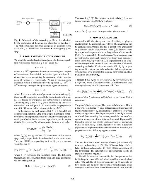
Theorem 1 (cf. [5]) The random variable η(f λ (y)) is an unbiasedestimator <strong>of</strong> MSE(f λ (y)), that is,E b {MSE(f λ (y))} = E b {η(f λ (y))}, (6)where E b {·} represents the expectation with respect to b.Fig. 1. Schematic <strong>of</strong> the denoising problem: ˜x is obtainedby the application <strong>of</strong> the denoising <strong>algorithm</strong> on the data y.The MSE estimation box then computes an estimate <strong>of</strong> theMSE <strong>of</strong> ˜x (i.e., SURE) as a function <strong>of</strong> λ knowing only y andf λ (y).2. PROBLEM FORMULATION AND SUREWe adopt the standard vector <strong>for</strong>mulation <strong>of</strong> a denoising problem:we measure noisy data y ∈ R N given by,y = x + b, (1)where x ∈ R N represents the vector containing the samples<strong>of</strong> the unknown deterministic noise-free <strong>signal</strong> and b ∈ R Ndenotes the vector containing the zero-mean white Gaussiannoise <strong>of</strong> variance σ 2 , respectively. We are given a denoising<strong>algorithm</strong> which is represented by the operator f λ : R N →R N that maps the input data y on to the <strong>signal</strong> estimate ˜x:˜x = f λ (y), (2)where λ represents the set <strong>of</strong> <strong>parameters</strong> characterizing f λ ;these should be adjusted to yield the best estimate <strong>of</strong> the <strong>signal</strong>[see Figure 1]. Our primal aim in this work is to optimizeλ knowing only y and ˜x = f λ (y) as illustrated by the “MSEestimation” box in Figure 1. To achieve this, we propose theuse <strong>of</strong> SURE as a reliable estimate <strong>of</strong> the true MSE.In the sequel, we will assume that f λ is a bounded andcontinuous operator (i.e., the input-output mapping is continuousand a small perturbation <strong>of</strong> the input necessarily yields asmall perturbation in the output). In particular, we do requirethat the divergence <strong>of</strong> f λ with respect to the data y given bydiv y {f λ (y)} =N∑k=1∂f λk (y)∂y k, (3)where f λk (y) and y k are the k th component <strong>of</strong> the vectorsf λ (y) and y respectively, is well-dened in the weak sense.Then the SURE corresponding to ˜x = f λ (y) is a randomvariable given byη(f λ (y)) = 1 N ‖y − f λ(y)‖ 2 − σ 2 + 2σ2N div y{f λ (y)}, (4)where ‖·‖ 2 represents the Euclidean norm. The followingtheorem, due to Stein, states that η is an unbiased estimate <strong>of</strong>thetrueMSEgivenbyMSE(f λ (y)) = 1 N ‖x − f λ(y)‖ 2 . (5)3. MONTE-CARLO SUREAs noted in (4), the divergence term, div y {f λ (y)}, playsapivotal role in the computation <strong>of</strong> SURE. The divergence canbe calculated analytically and has a closed <strong>for</strong>m expressiononly in some special cases such as when f λ is linear or whenf λ is a pointwise operator in an orthogonal trans<strong>for</strong>m domain[6–8]. For a general f λ , the evaluation <strong>of</strong> the divergence maynot be tractable analytically and worse, it may even be numericallyinfeasible, especially if f λ is implemented in an iterativefashion (as is the case with most variational or PDE-baseddenoising methods). We circumvent this difculty by proposinga novel technique that is based on the following theoremwhich allows us to estimate the required divergence (and thusSURE) <strong>for</strong> an arbitrary f λ .Theorem 2 Let f λ (z) be the output <strong>of</strong> f λ corresponding toz = y + b ′ ,whereb ′ is a zero-mean i.i.d random vector (thatis independent <strong>of</strong> y) with covariance ε 2 I.Then1div y {f λ (y)} = limε→0 ε 2 E b ′{b′ T (f λ (z) − f λ (y))}, (7)provided that f λ admits a well-dened second order Taylorexpansion.The pro<strong>of</strong> <strong>of</strong> this theorem will be presented elsewhere. This isa powerful result since (7) does not require any knowledge <strong>of</strong>the functional <strong>for</strong>m <strong>of</strong> f λ , thus making it applicable <strong>for</strong> a widevariety <strong>of</strong> <strong>algorithm</strong>s. The important point is that f λ is treatedas a black-box, meaning that we only need the output <strong>of</strong> theoperator irrespective <strong>of</strong> how it is implemented. Equation (7)<strong>for</strong>ms the basis <strong>of</strong> our Monte-Carlo approach <strong>for</strong> computingSURE <strong>for</strong> a general f λ . Since, in practice, the limit in equation(7) cannot be implemented due to nite machine precision, wepropose to use the following approximation:div y {f λ (y)} ≈ 1 ε 2 b′ T (f λ (y + b ′ ) − f λ (y)). (8)The idea is to add a small amount <strong>of</strong> noise (<strong>of</strong> variance ε 2 )to y and evaluate f λ (y + b ′ ). The difference f λ (y + b ′ ) −f λ (y) is then used according to (8) to obtain an estimate <strong>of</strong>the divergence. The schematics <strong>of</strong> implementing the rhs <strong>of</strong>(8) is illustrated in Figure 2.We will demonstrate numerically that the approximationin (8) is quite reasonable and yields excellent numerical results.The validity <strong>of</strong> the approximation in (8) depends onhow small ε can be made. In practice, we must select ε smallenough to mimic the limit, but still large enough so as to avoid906


