An exact method for computing the area moments of ... - IEEE Xplore

IEEE TRANSACTIONS ON PATTERN ANALYSIS AND MACHINE INTELLIGENCE, VOL. 23, NO. 6, JUNE 2001 633An Exact Method for Computing the AreaMoments of Wavelet and Spline CurvesMathews Jacob, Student Member, IEEE, Thierry Blu, Member, IEEE, andMichael Unser, Fellow, IEEEAbstractÐWe present a method for the exact computation of the moments of a region bounded by a curve represented by a scalingfunction or wavelet basis. Using Green's Theorem, we show that the computation of the area moments is equivalent to applying asuitable multidimensional filter on the coefficients of the curve and thereafter computing a scalar product. The multidimensional filtercoefficients are precomputed exactly as the solution of a two-scale relation. To demonstrate the performance improvement of the newmethod, we compare it with existing methods such as pixel-based approaches and approximation of the region by a polygon. We alsopropose an alternate scheme when the scaling function is sinc…x†.Index TermsÐArea moments, curves, splines, wavelets, Fourier, two-scale relation, box splines, wavelet-Galerkin integrals.æ1 INTRODUCTIONMOMENTS are standard descriptors of the shape of anobject [1], [2], [3]; they easily yield features that areinvariant to translation and rotation [4] or, more generally,to affine transformations, which makes them useful toolsfor pattern recognition. In the standard formulation, theyare computed as surface integrals which requires rasterscanning through the image. However, there are manyinstances where the boundaries of objects are described byparametric curves. This is the case, for example, when theobjects are detected using parametric snakes which arerepresented using B-spline [5], [6], [7], [8] or wavelet basisfunctions [9], [10]. Another simple case is when the region isdescribed as a polygon [11].In this paper, we address the problem of computing thearea moments of objects described by such parametriccurves when the basis functions are scaling functions. Thepopular wavelet curve descriptors also fall into this class.The originality of our approach is that the computation isexact and also more direct than the conventional pixelbasedmethod which requires an explicit labeling of theinner region of the curve prior to computation. Moreover,the pixel-based schemes suffer a low accuracy due to theloss of subpixel details in the rasterizing process. Also, theerror in the area-based computation of moments isdependent on the orientation of the shape.Since a polygon can be represented in terms of linearsplines, the computation of moments by approximating theshape as a polygon [11], [12], [13] is a particular case of ourapproach. While the polygon method can be made asaccurate as desired by increasing the number of segments,the convergence is slow because of the low approximation. The authors are with the Biomedical Imaging Group, Swiss FederalInstitute of Technology, Lausanne, CH-1015 Lausanne, EPFL, Switzerland.E-mail: {mathews.jacob, thierry.blu, michael.unser}@epfl.ch.Manuscript received 7 June 2000; revised 6 Feb. 2001; accepted 2 Mar. 2001.Recommended for acceptance by S. Sarkar.For information on obtaining reprints of this article, please send e-mail to:tpami@computer.org, and reference IEEECS Log Number 112243.order of linear splines. Moreover, it is not suitable forcomputing the curvature, which is an interesting shapefeature as it is invariant to rotation and translations, and canbe easily normalized to scale changes. This motivates us toinvestigate higher order schemes where the curve isrepresented by smoother basis functions such as B-splinesand other scaling functions that appear in wavelet theory[14], [15]. These type of basis functions also occur naturallywhen one seeks multiresolution representation of curveswhich are well suited for pattern recognition and shapesimplification [16], [10].The paper is organized as follows: In Section 2, we showhow Green's Theorem can be used for the computation ofthe area moments of a parametric curve. In Section 3, weconsider the computation of the moments of such a curverepresented in spline or wavelet bases. Here, we alsodiscuss the properties of the multidimensional kernel usedin the computation of moments. In Section 4, we give theimplementation details of the moment computation. In thefollowing section, we deal with the precomputation of thekernel. In Section 6, we present an alternate implementationthat works for any order moments, but it is rigorously exactonly when the scaling function is sinc…x†. This is especiallyinteresting because it makes our method applicable to theFourier representation of curves as well. In the last section,we compare the new method with the existing schemessuch as approximation using polygons and rasterizing.2 PRELIMINARIES2.1 Computation of Moments UsingGreen's TheoremGreen's Theorem relates the volume integral of thedivergence of a vector field in a closed region to theintegral of the field over the surface enclosing it. In thissection, we show how it can be used to compute themoments of an area enclosed by a curve.0162-8828/01/$10.00 ß 2001 IEEE

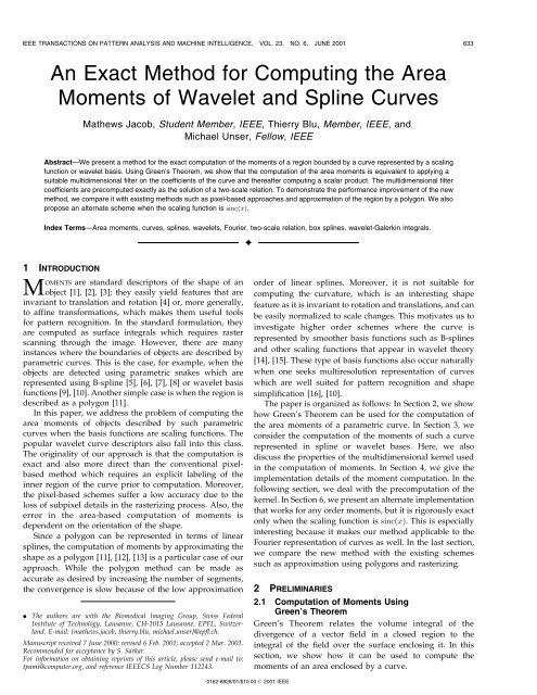
634 IEEE TRANSACTIONS ON PATTERN ANALYSIS AND MACHINE INTELLIGENCE, VOL. 23, NO. 6, JUNE 2001Consider a closed region V, bounded by a surface S.Green's Theorem states that, for any vector field F,ZZ…r:F† dV ˆ F:dS;…1†Vwhere dS is the unit vector pointing out of the surface S.Assuming the volume has a constant cross-section boundedby the curve C and that the variation of the field along thez-direction is zero, we can restrict the theorem to twodimensions as,Z @F xS @x ‡ @F Iydxdy ˆ …F y dx F x dy†: …2†@yCThe first integral is evaluated over the area S enclosed bythe curve and the second one along the curve C in theclockwise direction. The computation of the momentsinvolves the evaluation of the integral R S xm :y n :dxdy on thesurface bounded by the curve. This, by (2), is equivalent toII m;n ˆCSx m y n‡1n ‡ 1 dx;with F ˆ e y … xm y n‡1n‡1 †; e y denotes the unit vector along they direction. Note that the choice of F is not unique. Wechoose the vector field F that makes the computationsimple. Another possible choice that has the same computationalcomplexity is F ˆe x … xm‡1 y nm‡1 †.2.2 Parametric Representation of a CurveA curve in the x Ð y plane can be represented in terms of anarbitrary parameter t as r…t† ˆ…x…t†;y…t††. If the curve isclosed, as discussed in the paper, the functions x…t† and y…t†are periodic.When the curve C is represented as above, r…t† can beapproximated efficiently as linear combinations of somebasis functions, which makes the representation compactand easy to handle.In this paper, we mainly focus on the representation ofthe function vector r…t† in a scaling function basis asr…t† ˆ X1kˆ1b k '…t k†:Here, b k denotes the sequence of vector coefficients givenby b k ˆ…c k ;d k †. If the period, M, is an integer, we haveb k ˆ b k‡M . This reduces the infinite summations towherer…t† ˆXM1kˆ0' p …t† ˆ X1kˆ1b k ' p …t k†;'…t k:M†:In the context of wavelets, ' is called the scaling function; itsatisfies the two-scale difference equation'…t† ˆXh…k†'…2t k†;…7†k…3†…4†…5†…6†Fig. 1. Example: A polygon and its parametric representation.where h…k† is the mask of the corresponding refinementfilter [14]. The scaling function representation enables us tohave local control of the contour, which is desirable in manyapplications. It also permits a multiresolution representationof the curve [9], [17]. Moreover, the scaling functionrepresentation is affine-invariant; an affine transformationof the curve is achieved simply by transforming thecoefficient vector b k ;kˆ 0; 1; ...;M 1. This is because ofthe linearity of the representation and the partition of unitycondition:X 1kˆ1'…t k† ˆ1;which is satisfied by all valid scaling functions in wavelettheory. Among the scaling functions, a case of specialinterest is ' ˆ n , where n is the causal B-spline of degree n[18] defined by its Fourier transform^ s …!† ˆ 1 s‡1 ej!: …9†j!This yields spline curves which are frequently used incomputer graphics [19] and computer vision [6], [20], [21].We now consider a simple example to illustrate this kindof curve representation. Given in Fig. 1 is a polygon and itsparametric representation. The dotted lines show the linear…8†

JACOB ET AL.: AN EXACT METHOD FOR COMPUTING THE AREA MOMENTS OF WAVELET AND SPLINE CURVES 635B-spline basis functions, 1 …t k† (tent function), multipliedby the corresponding coefficients.The description of C in the scaling function basis isequivalent to a periodized wavelet representation [9]. Thisimplies that, if we have a wavelet description of the curve,the scaling function coefficients at any scale can be obtainedfrom the wavelet coefficients using the fast reconstructionequation described in [22]. Hence, the theory is sufficientlygeneral to include the wavelet curve descriptors as well.The representation of the curves in a sinc basis also fallsin this class, as sinc is a valid scaling function. Thedescription of the curve in the sinc basis as (5) is notefficient, as sinc has an infinite mask unlike most of thewidely used scaling functions. It is well known (c.f. [23])that the sinc interpolation of a periodic signal can beformulated into a numerically stable and efficient expressionasr…t† ˆ XLkˆLb k expj2kt ; …10†Mwhere 2L ‡ 1 ˆ M, assuming M to be odd. A similarexpression is obtained for even M as well. Here, b k is thediscrete Fourier transform of the vector sequence r…k†. Notethat (10) provides the Fourier series description of thecurve, which is frequently used for the representation ofclosed curves [24], [25].2.3 Differentiation of Scaling FunctionsWe will use the property that the kth derivative of a scalingfunction ' can be expressed as [26]' …k† …x† ˆ k ' fkg …x†;…11†where ' fkg …x† denotes the scaling function whose mask isgiven by H fkg 2 k…z† ˆ1 ‡ z 1 H…z†;H…z† is the mask of '. denotes the backward differenceoperator, defined as …x† ˆ…x†…x 1†.The relation (11) follows from the fact that any mth orderscaling function can be written as^'…!† ˆ 1 mej!^…!†;j!|‚‚‚‚‚‚‚‚{z‚‚‚‚‚‚‚‚}^ m1 …!†where is a refinable distribution which doesnot satisfythemHpartition ofunity.The mask of ' is H…z† ˆ 1‡z12…z†.m1‡zNote that12 is the mask of m1 and H the mask of .Differentiating ' with respect to x, k number of times(k m) yields' …k† …x† ! F … j! † k ^'…!† ˆ 1 e j! k 1 e j! mk^…!†j!|‚‚‚‚‚‚‚‚‚‚‚‚‚‚‚{z‚‚‚‚‚‚‚‚‚‚‚‚‚‚‚}^' fkg …!†!F 1 k ' fkg …x†: …12†Thus, the mask of ' fkg …x† isH fkg …z† ˆ 1 ‡ mk z12 kH …z† ˆ21 ‡ z 1 H…z†:3 COMPUTATION OF THE MOMENTS OF AN AREABOUNDED BY A PARAMETRIZED CURVETo facilitate the understanding of our method, we first givea detailed derivation of the formula for the area of theregion bounded by the curve. We then extend ourformulation to the general case.3.1 Computation of the AreaFor the parametric representation of the curve, the area ofthe region is given byZ MI 0;0 ˆ y…t† dx…t† dt:…13†0 dtWhen the curve is described in a scaling function basis as in(5), we havewhereXM1 Z MI 0;0 ˆ d i c ji;jˆ00' p …t i†' 0 p …t j†dt; …14†' 0 p …t† ˆd' p…t†:dtSubstituting for ' 0 p…t† from (6), we getXM1 Z 1I 0;0 ˆ d i c j ' p …t i†' 0 …t j†dt;i;jˆ0which is equivalent to1…15†XM1 Z 1I 0;0 ˆ d i c j ' p …t i ‡ j†' 0 …t†dti;jˆ0 1|‚‚‚‚‚‚‚‚‚‚‚‚‚‚‚‚‚‚‚‚{z‚‚‚‚‚‚‚‚‚‚‚‚‚‚‚‚‚‚‚‚}g p 0 …ij† : …16†Again, substituting for ' p from (6), we get the kernel g p 0…l† asthe M periodized version ofg 0 …l† ˆZ 11' 0 …t†'…t l†dt…17†as g p 0…l† ˆP1kˆ1 g 0…l ‡ k:M†. With the simplification (11),the above equation becomesandf 0 …x† ˆg 0 …l† ˆf 0 …l†;Z 11' f1g …t†'…t x†dt:…18†…19†Note that, if '…t† ˆ'… t†, then f 0 …x† can be written as the convolution ' f1g ' … ‡ x†. We prefer to represent thekernel g p in terms of f due to its nice properties, discussedlater.

636 IEEE TRANSACTIONS ON PATTERN ANALYSIS AND MACHINE INTELLIGENCE, VOL. 23, NO. 6, JUNE 2001Z 1Substituting for ' 0 p …t† from (6), we get Both these properties together imply 2……m ‡ n ‡ 1†!†relations, which are used to accelerate the computationFor the example given in Fig. 1, we haveI m;n ˆ 1 XXc k c ‰mŠ ‰n‡1Ši d j ' p …t i 1 † ...g 0 …l† ˆ 0 1 n ‡ 1…l ‡ 2† ˆ… 2 k2R i2R m‡11…25†j2R†…l ‡ 2†g 0 : …0:5; 0; 0:5†; l 2f1; 0; 1g;' p …t i m †' p …t j 1 † ...' p …t j n‡1 †' 0 …t k†dt:where n is the causal B-spline function of degree n. The integral in the above equation is equivalent toRNow, for the polygon, c…k† : …1; 1; 6; 8; 7; 4† and d…k† :11 '0 …t†' p …t‡ki 1 †...' p …t‡ki m †' p …t‡kj 1 †...' p …t‡kj n‡1 †dt : …26†|‚‚‚‚‚‚‚‚‚‚‚‚‚‚‚‚‚‚‚‚‚‚‚‚‚‚‚‚‚‚‚‚‚‚‚‚‚‚‚‚‚‚‚{z‚‚‚‚‚‚‚‚‚‚‚‚‚‚‚‚‚‚‚‚‚‚‚‚‚‚‚‚‚‚‚‚‚‚‚‚‚‚‚‚‚‚‚}…1; 6; 8; 5; 1; 0†. Hence, by (16), we haveg p m‡n …ik;jk†I 0;0 ˆ 1 h…6; 8; 5; 1; 0; 1†; …5; 7; 1; 4; 6; 3†iHence, the …m; n†th order moment is2ˆ 42 units:I m;n ˆ 1 XXc k c ‰mŠ i d ‰n‡1Š j g pn ‡ 1m‡n…i k; j k†: …27†k2R i2RHere, hx 1 ;x 2 i stands for the `2 inner product given byj2RPk x 1…k†x 2 …k†.tu3.2 General FormulaAs in the case of the area, the kernel g p is obtained by theHaving shown how to compute the area, we proceed on to M-periodization ofZthe general case. The formula for the computation of the1g m‡n …k† ˆ ' 0 …t†'…t k 1 †::'…t k m‡n‡1 †:dt;general moments are given by the following theorem:1…28†Theorem 1. Let C be a closed curve in the x-y plane represented where k 2 Z m‡n‡1 . Expressing ' 0 in terms of ' f1g , we getin the parametric form in a periodized scaling function basis asg m‡n …k† ˆf m‡n …k†f m‡n …k 1†; …29†(4). Then, the …m; n†th order area moment of the region S,wherebounded by the curve C, given byZZ1I m;n ˆ x m y n fdxdy for m; n 0 …20† m‡n …x† ˆ ' f1g …t†'…t x 1 †::'…t x m‡n‡1 †dt; …30†1Swhere x ˆ…xcan be computed as1 ;x 2 ...;x m‡n‡1 †2 R m‡n‡1 . The kernel f hasmany interesting properties, which are discussed next.I m;n ˆ 1 XXc k c ‰mŠ i d ‰n‡1Š j g pn ‡ 1m‡n…i k; j k†; …21† 3.3 Properties of the KernelÐfk2R i2R m‡1j2R nwhere R is the integer range ‰0...M 1Š. The kernel g p m‡n in(21) isZ 11. Finite Support. As the kernel is an integral ofproducts of the translates of finitely supportedfunctions, it has a finite support as well. If thescaling function is continuous and has a supportg p m‡n…k† ˆ ' 0 …t† ' p …t k 1 † ...' p …t k m‡n‡1 † dt: …22† ‰0;NŠ, then the kernel will be supported on the1integer points in the intervalHere, c ‰mŠ stands for the m-times tensor product 1 c I ˆ‰N ‡ 1;N 2Š...c ... c and i k denotes the sequence‰N ‡ 1;N 2Š‰N ‡ 1;N 2Š:…31†…i 1 k; i 2 k; ...i m‡1 k†:Proof. For a parametric curve, the evaluation of the …m; n†thorder moment given by (20) can be reduced to2. Symmetry. The fact that the kernel is obtained fromthe integration of similar translated scaling functionsintroduces a lot of symmetry. As (30) is symmetricI m;n ˆ 1 Z Mx m …t†y n‡1 …t† dx…t†with respect to the parameters k 1 ;k 2 ;::, interchangingthem will not affect the value of the kernel. Thisdt …23†n ‡ 1 0dtimpliesby (3). When the curve is described in a scaling functionf…k† ˆf… i …k††;…32†basis, we havewhere i indicates all possible …m ‡ n ‡ 1†! permutationoperators. In addition, if the scaling functionsI m;n ˆ 1 XXZ Mc k c ‰mŠ ‰n‡1Ši d j ' p …t i 1 † ...n ‡ 1k2R i2R m‡10are symmetric as in the case of splines, we have…24†j2R n' p …t i m †' p …t j 1 † ...' p …t j n‡1 †' 0 p …t k†dt:f…k† ˆf…k†:…33†1. c ‰0Š is defined as the neutral element c ‰0Š c ‰mŠ ˆ c ‰mŠ .of the kernel as well as themoments.

JACOB ET AL.: AN EXACT METHOD FOR COMPUTING THE AREA MOMENTS OF WAVELET AND SPLINE CURVES 6373. Two-Scale Relation. We now show that the kernelsatisfies a two-scale relation, which is the key to ourcomputational approach. This property follows fromthe fact that the scaling functions '…t† and ' f1g …t†,from which the kernel is derived, satisfy two-scalerelations. If we consider (30) and rewrite the ' and' f1gin terms of the corresponding two-scale relations(cf. (7)), we getf m‡n …k† ˆXl2 Z m‡1 H m‡n …l†:f m‡n …2k l†;…34†where k 2 Z m‡1 . The mask H in the above equationisXH m …l 1 ;l 2 ; ::; l m †ˆ1h 1 …k†:h…k l 1 †::h…k l m †:2k…35†The z-transform of the mask is given byH m …z 1 ;z 2 ; ::; z m †ˆ12 H 1… Q mkˆ1 z k† Ymkˆ1H…z 1k †: …36†It is this property that enables us to compute thekernels exactly, by solving a linear system ofequations. This technique, which is discussed later,is analogous to the computation of the integer (ordyadic rational) samples of a scaling function fromthe transition operator [14].Note that a scaling relation similar to (34) wasalso considered by mathematicians in the context ofthe wavelet-Galerkin method for the computation ofintegrals involving products of scaling functions andtheir derivatives [27], [28]. The work of Dahmen andMiccheli is essentially theoritical; Restrepo and Leafconcentrated on numerical issues and proposed asolution which is equivalent to the computation ofour kernel g m instead of f m . This slightly complicatesthe approach and also increases the dimensionalityof the problem; this issue is discussed further inSection 5.1.The above mentioned properties imply that the kernelcan be computed exactly for any finitely supported scalingfunction, as discussed in Section 5. In the next section, wewill give some examples for the kernels when the scalingfunctions are B-splines.3.4 Examples with SplinesSplines possess nice approximation properties. The B-splineshave the maximum approximation order among the class offunctions that satisfy a two-scale relation with a givensupport. Hence, they give better local control of the contour.Moreover, they are symmetric, which facilitates the computationof the kernel and moments as discussed before. So, it isworthwhile to analyze the properties of the kernels for aspline representation of the curve. For the results used in thissection, refer to [18].We consider causal B-splines, as they satisfy a two-scalerelation for all orders. The refinement filter for a B-spline ofdegree n is the binomial filterh…k† ˆ 1 n ‡ 12 n : …37†kIf we choose s , a B-spline of degree s, as ', then' f1g ˆ s1 ; that is a spline of degree s 1. Hence, thekernel f as given by (30) is a box spline [29] sampled at theintegers. In particular,f 0 …k† ˆ 2s …k ‡ s ‡ 1†:…38†The spline functions have a closed-form representation inthe Fourier domain, which the kernels also inherit. Bytaking the continuous Fourier transform of (30), when thescaling function is a B-spline, we get^f s n …!†; ! 2 Zn ˆ ^ s1 …j!j† Ynkiˆ1^ s …! i †;…39†where j!j stands for P njˆ1 ! j. By using Poisson's formulaX^f n s 1 X…! ‡ 2k† ˆ fn s 2…k†e2j!k ; …40†we get the discrete Fourier transform of the kernel as the2-periodized version of (39).We give some examples of kernels for the computation ofthe first three moments when we have a linear splinerepresentation. For linear splines, the kernel f m1…k 1 ;k 2 ; ...;k m † is supported in the interval ‰1; 0Š‰1; 0Š ...‰1; 0Š. The kernels arekf 0 …k 1 †; k 1 2f1; 0g : 1 ‰1 1Š; …41†2f 1 …k 1 ;k 2 †; k 1 ;k 2 2f1; 0g : 1 6 1 2; …42†2 18 f 2 …1;k 2 ;k 3 †; k 2 ;k 3 2f1; 0g : 1 12 1 1>:1 1…43†It is interesting to see that the computation of the momentsusing the linear spline kernel is the same as when thepolygon is triangulated in a specified way and the momentsof individual triangles added up as in [11].We also give the kernel f 0 for the cubic splinerepresentation.1f 0 …k 1 †; k 1 ˆ3; ...2: :‰1; 57; 302; 302; 57; 1Š: …44†720The higher order kernels are omitted due to spaceconstraints. They can be downloaded from http://bigwww.epfl.ch/jacob.4 IMPLEMENTATIONIn this section, we analyze equation (21) and simplify it forfaster computation. We start with the simplest case: the areaof the region.

638 IEEE TRANSACTIONS ON PATTERN ANALYSIS AND MACHINE INTELLIGENCE, VOL. 23, NO. 6, JUNE 2001The area bounded by the curve (cf. (15)) is computed asI 0;0 ˆ XM1c p XN2kkˆ0 lˆN‡1d p k‡l g 0…l†;…45†where g 0 is given by (17). The sequences c p k and dp k areM-periodized versions of the coefficients c k and d k withrespect to the period M. This is simply because convolvinga nonperiodized sequence with a periodized kernel isequivalent to convolving a periodized sequence with anonperiodized kernel. We have also reduced the range ofsummation of the inner sum to N ‡ 1 to N 2, which istypically much less than the range 0 to M 1. Similarly, forthe higher order moments all the summations, except theouter one, are in the range N ‡ 1 to N 2.From (45), we see that the computation of the areainvolves just a filtering operation by g…l† ˆg T …l†, followedby an inner product. This can be written as,I 0;0 ˆhc p ;g T 0 dp i;…46†wherePh:; :i stands for the inner product hc; di ˆM1kˆ0c…k†d…k†. With a similar notation, the computationof the other moments are given asI m;n ˆ hcp ;g T m‡n …cp‰mŠ d p‰n‡1Š †in ‡ 1…47†ˆ hdp ;g T m‡n …cp‰m‡1Š d p‰nŠ †i: …48†m ‡ 1As the …m ‡ n ‡ 1†-D sequence is separable, the filteringoperation is much simpler than the usual …m ‡ n ‡1†-dimensional filtering.The complexity in the computation of the moment I m;n isM:…2N 2† …m‡n‡2† , without taking the symmetries intoaccount. Thus, for basis functions with small support andreasonable m and n, the complexity is quite managable.5 COMPUTATION OF THE KERNELIn this section, we propose two schemes for computing thekernel. An exact space domain scheme and an approximateone in the Fourier domain.5.1 Exact MethodIn this scheme, we compute the kernels in space domainmaking use of the properties of kernels discussed before.We start with the computation of f 0 and later extend it tothe general case. Making use of the finite support property,the two-scale relation (34) can be rewritten in the matrixform as,A 0 :f 0 ˆ f 0 ;…49†where A 0 is the square matrix with coefficients ‰A 0 Š k;l ˆH 0 …2k l† and f 0 is the vector whose elements are f 0 …n†. Asthe support of f 0 is ‰N ‡ 1;N 2Š, the indices of A 0 runfrom N ‡ 1 to N 2.It can be seen from (49) that f 0 is an eigen-vector of thematrix A 0 , with eigen-value 1. Solving for f 0 is equivalent tosolving for a vector which falls in the nullspace of …A 0 I†,where I is the identity matrix. Since f 0 6ˆ 0, A 0 must havethe eigen-value 1, which is in general single. This providesf 0 up to a constant which is further set by the normalizationidentityXf 0 …k† ˆ1;…50†kwhich can be seen from (19). This is because the function '…x†has at least an approximation order of one [14], which impliesPk '…x ‡ k† ˆ1. One of the equations in …A 0 I†:f 0 ˆ 0 canbe substituted for by the (50) to yield the system of equationsgiven byB:f 0 ˆ y;…51†B is the matrix obtained by substituting one of the rows of…A 0 I† with the row vector ‰1; 1; ...; 1Š and y is given by‰0; 0; 0...; 0; 0; 1Š T c.f [30]. Now, B is a full rank matrix and,hence, the eigen-vector f 0 can be solved by matrix inversion.To represent the two-scale relations of the higher orderkernels in the matrix form, we introduce a one-to-onefunction : ‰N ‡ 1;N 2Š m 7!‰0; …2N 2† m 1Š. Usingthis function, (34) can be rewritten asf m … 1 …k†† ˆ…2N2†Xm‡1 1lˆ0 H m 2 1 …k† 1 …l† fm 1 …l† ;which is a linear system of equations. This can be written inthe matrix form asA m f m ˆ f m ;…52†where ‰A m Š i;j ˆ H m … 2 1 …i† 1 …j†† and f m …i† ˆf … 1 …i††.This equation is of the same form as (49) and can be solvedinPthe same way, with the normalization constrainti f m…i† ˆ1.Let us now compare our computational solution with themethod developed for computing g m in the context ofwavelet-Galerkin approach [27]. For a scaling function ofsupport N, the kernel g m is zero outside the intervalI 0 ˆ‰N ‡ 1;N 1Š...…53†‰N ‡ 1;N 1Š‰N ‡ 1;N 1Š:as compared to f m whose support is given by (31). Thus, thedirect computation of g m involves a linear system with…2N 1† m variables as compared to …2N 2† m for f m in ourcase. For 3-dimensional kernels involving cubic splines, weachieve a 40 percent reduction in the number of equations.As the computational complexity in inverting a linearsystem is proportional to the third power of the number ofequations, this implies a performance improvement ofaround 5 times. The approach becomes even more rewardingfor higher order kernels. Moreover, the normalizationconstraint (50) that we use to make the system full rank ismuch more straightforward than the corresponding relationfor the derivative functions.Note that this simplification is covered by Dahmen andMichelli's general theory for integrals of multidimensionalscaling functions [28]. This is because the mask of anymth order 1 D scaling function can be always factored asproposed in [28, Corollary 3.3]. In the case of wavelet-Galerikin integrals, the performance improvement can evenmore substantial depending on the number of derivatives.

JACOB ET AL.: AN EXACT METHOD FOR COMPUTING THE AREA MOMENTS OF WAVELET AND SPLINE CURVES 6395.2 Approximate Method for SplinesBecause the spline kernel has a closed-form expression inthe frequency domain, the kernel can be obtained by takingthe inverse DFT of the above mentioned Fourier transform(40) sampled at an appropriate rate; we make use of thefinite support property of the kernel. As sinc is a decayingfunction, the periodization of the Fourier transform may beapproximated with an appropriately truncated sum toachieve any desired accuracy. This is because we can havean upper bound for the error that is a decreasing function ofthe summation range. Moreover, the symmetries of thekernel discussed before may be used for the efficientcomputation of the box spline kernels as in [31].However, this technique, besides being approximate, canbe used only for scaling functions that have a closed formexpression in the frequency domain, i.e., splines in practice.This scheme may be useful to precompute the spline kernelsfor very high order moments, where the exact scheme canbe computationally expensive.6 COMPUTATION OF THE AREA MOMENTS USINGRIEMANN SUMSAn alternate approach to compute the moments is toapproximate the integral (3) by a Riemann sum:1MP1I m;n ˆ…n ‡ 1†P : X‰x int …l=P †Š m :‰y int …l=P †Š n‡1 :‰x 0 int …l=P †Š;lˆ0…54†where P is an appropriate oversampling factor. We show inthis section that this quadrature formula is exact when thecurves are described in a sinc basis. For other representations,it can be used for the approximate computation ofhigher order moments.6.1 Sinc Representation of the CurveA curve represented in a sinc basis also falls into theframework of Theorem 1 because sinc…x† is a valid scalingfunction. However, computing the moments as described inSection 4 is expensive as the mask of the sinc function is notfinitely supported. We remind the reader that the representationof a periodic signal in the sinc basis is equivalentto the Fourier representation as seen in (10).In this particular case, the moments can be computedexactly and more efficiently using (54), where the oversamplingfactor, P , is any integer greater than m‡n‡22.Proposition 1. The quadrature formula (54) is exact for the sincrepresentation provided that P d m‡n‡22e.The continuously defined functions x int …t† and y int …t† areobtained by interpolating the sample values of the curve atthe integers, using the periodized sinc function. Thecomputation is exact because we implicitly assume thatthe functions x…t† and y…t† are bandlimited functions, withbandwidth B ˆ 2.Proof. The integral (3) can be considered as an L 2 …0;M† innerproduct of two functions, which are d m‡n‡22e and b m‡n‡22cfold 2 products of the corresponding band-limited2. bxc and dxe denote the floor and the ceil operators, operating on afraction x to yield the lower and upper integers that bound x.functions. Hence, they are bandlimited by B 0 ˆBd m‡n‡22e and B 00 ˆ Bb m‡n‡22c, respectively. So, thesefunctions are exactly represented in the basis fsinc…Pxk†; 8k 2 Zg, where 2P B 0 . Because the sinc basis isorthogonal, the L 2 …0;M† inner product is equivalent to the`2 …0;MP1† inner product. Hence, it is sufficient tocompute the discrete summation instead of the integral.Finally, the sinc function is interpolating, so that thecoefficients of the basis functions are the resampledcurve values and, hence, the result (54).tuUsing the equivalence of the sinc and the Fourierrepresentations, we can compute the interpolated samplesefficiently with a MP point inverse FFT of the Fouriercoefficients c k and d k .We will compare the sinc moment estimator with thescaling-function-based moment estimator in the next section.One disadvantage of the Fourier(sinc) representationof curves is the loss of local control property that we werehaving with the finitely supported scaling functions.The complexity in the computation of the momentsin this scheme is MP…3 log…MP†‡…m ‡ n ‡ 2††. Here,3MP log…MP† is the cost of the inverse FFT of thesequences c k , d k , and k:c k , and …m ‡ n ‡ 2†MP correspondsto the multiplications.6.2 Spline Representation of the CurveThe quadrature formula (54) is also applicable to the splinerepresentation, provided that the functions x int …t† and y int …t†are obtained by interpolating the integer sample values,using the corresponding B-spline functions. This scheme isno longer exact, but it may be a viable alternative forcomputing the higher order moments. The necessarycondition for the computation to be reliable is that theFourier transform of the B-spline function is essentiallybandlimited to 2P, where P is the oversampling factor.The error in the moments computed with the approximatemethod is, thus, proportional to the residual energy of theB-spline function in the corresponding outband. As theFourier transform of the B-spline is a decaying function ofthe frequency, the error will be a decaying function of P aswell. Thus, any desirable accuracy may be achieved bychoosing P sufficiently large.The complexity of the spline quadrature formula is O…M…m ‡ n ‡ 2†…m ‡ n ‡ 2 ‡ 3N†P†, where M…m ‡ n ‡ 2†P isthe total number of resampled points. The evaluation of thespline representation requires N multiplications to obtainone resampled point from the corresponding B-splinerepresentation. Then, the computation of the discrete sumcosts m ‡ n ‡ 2 multiplications per resampled point. Interestingly,the approximate scheme will give better results forhigher order splines as these functions will becomebandlimited as the order tends to infinity [32].7 EXPERIMENTS AND RESULTSIn this section, we compare the new technique with theexisting ones: approximation using polygons and rasterizing.We first consider the exact scheme proposed inSection 4. We try to estimate the parameters of a known

640 IEEE TRANSACTIONS ON PATTERN ANALYSIS AND MACHINE INTELLIGENCE, VOL. 23, NO. 6, JUNE 2001Fig. 2. Comparison of moment estimators.ellipse and choose the relative error in the parameters as thecriterion of comparison.Our preferred choice is to represent the curve in a cubicB-spline basis due to its nice approximation properties andminimum curvature properties. To compare it with theapproximation of the region as a polygon, the ellipse issampled uniformly and the samples are interpolated usingthe two techniques (linear and cubic splines). The averagerelative error in the three centered second order momentsversus the number or samples are plotted in Fig. 2. It can beseen that the relative error is much smaller for the cubicspline interpolation even at low sampling rates and that itexhibits a faster decay.In the traditional scanning approach, the ellipse isscanned along the x and y axes with a step size and themonomials are computed at the grid points assigned to theinterior of the curve. Fig. 3 shows the pdecay of the averageArearelative error for an ellipse versus for three different4. Estimated ellipse for a real image.orientations. The plot clearly shows the dependence of theaccuracy on the orientation of the ellipse.It can be seen that to achieve a relative error of0:1 percent the interior of the ellipse has to be sampled atabout 3,600 points, whereas to achieve the same error usingthe cubic spline interpolation we need only around ninepoints on the curve. In comparison, the polygon method(linear spline) requires more than 40 samples to have asimilar error. More interesting is the case when the interiorof the ellipse has to be sampled at about 2:5 10 5 points toachieve an error of 0:002 percent while the cubic splinesrequire only 25 samples to achieve the same accuracy. InFig. 4, we show the ellipse corresponding to the secondorder moments of the central structure in the image. Thecontour of the object was estimated using a snake wherethe curve was represented parametrically in terms of cubicB-splines; the moments are computed using our algorithm.Note that the fit is astonishingly good.Fig.Fig. 3. Variation of error versus 1 in a raster scan moment estimator.Fig. 5. Shape of corpus callosum represented using a cubic B-splinecurve with 20 knot points.

JACOB ET AL.: AN EXACT METHOD FOR COMPUTING THE AREA MOMENTS OF WAVELET AND SPLINE CURVES 641Fig. 6. Comparison of Fourier Estimator with cubic spline estimator.Having observed that the cubic spline estimator performsbetter than the polygon method, we now compare itwith the Fourier (sinc) technique proposed in Section 6. It isnot fair to use the ellipse as we did before because it can berepresented exactly in a Fourier series representation withL ˆ 2. So, we choose the real shape of corpus callosumshown in Fig. 5, represented in a linear spline basis with39 knot points as the reference shape. This shape wasresampled at different rates and these points were interpolatedusing cubic B-spline and Fourier representations,respectively. The moments of the corresponding curveswere calculated using the respective algorithms discussedbefore. Fig. 6 shows the decay of the relative error with theresampling rate for both representations. We observe thatthe spline estimator is better than the Fourier estimator forsmall sampling rates, while the Fourier estimator performsbetter at very high sampling rates (typically more than eighttimes the number of points used for the description of C). Inthe example considered, the Fourier method performsbetter when the shape of corpus callosum is representedwith around 312 samples.To evaluate the performance of the approximate schemeintroduced in Section 6.2, we now consider the case wherethe corpus callosum is represented by a cubic B-spline curvewith 20 knot points. The relative error in the computation ofthe second order moments by the quadrature formula as afunction of its relative computational complexity (proportionalto P) is shown in Fig. 7; here, the reference method isthe kernel-based computation, which is exact. Our resultsindicate that, for the second order moments, the error of thequadrature formula is quite substantial (e.g., 9.4 percent).Thus, it is not advantageous for computing the lower ordermoments. However, the quadrature formula will eventuallystart to pay off for higher order moments, because its costincreases only quadratically with the degree as compared toexponentially for the kernel-based method.8 CONCLUSIONIn this paper, we have presented a new approach for thecomputation of the moments of a curve described in awavelet or scaling function basis. It is especially usefulfor objects detected using parametric snakes. The mainFig. 7. Relative error versus relative computational complexity.advantages of the proposed scheme over the conventionalmethods are:. the exactness of the computation,. its independence of the orientation of the shape, and. the consistency with the snake model and the factthat it is the most direct method available.In addition, the method is reasonably fast and easy toimplement.We recommend using our exact kernel-based approachfor computing the lower order moments (typicallym ‡ n 2) for which the kernels are available. For higherorder moments, we have proposed a quadrature formulathat approximates the continuous integrals with Riemannsums. The latter method is exact for the sinc basis functions;otherwise, it can be made as accurate as desirable byresampling the model at a finer rate (P sufficiently large).ACKNOWLEDGMENTSThe authors would like to thank the anonymousreviewer for pointing us to references [28] and [27] onthe wavelet-Galerkin method which deal with thecomputation of wavelet related integrals. This workwas supported by the Swiss National Science Foundationunder grant 2100-053540.REFERENCES[1] S. Rad, K.C. Smith, and B. Benhabib, ªApplication of Moment andFourier Descriptors to the Accurate Estimation of Elliptical ShapeParameters,º Proc. IEEE Int'l Conf. Acoustics, Speech, Signal Process,vol. 4, pp. 2465±2468, 1991.[2] R. Desai, R. Cheng, and H.D. Cheng, ªPattern Recognition byLocal Radial Moments,º Proc. 12th IAPR Int'l Conf. PatternRecognition, 1994.[3] K. Tsirikolias and B.G. Mertzios, ªStatistical Pattern RecognitionUsing Efficient Two-Dimensional Moments with Applications toCharacter Recognition,º Pattern-Recognition, vol. vol. 26, pp. 877±882, 1993.[4] L.X. Shen and Y.L. Sheng, ªNoncentral Image Moments forInvariant Pattern Recognition,º Optical Eng., vol. 34, no. 11,pp. 3181±3186, 1995.[5] P. Brigger, J. Hoeg, and M. Unser, ªB-Spline Snakes: A FlexibleTool for Parametric Contour Detection,º IEEE Trans. Image Process,vol. 9, pp. 1484±1496, Sept. 2000.

642 IEEE TRANSACTIONS ON PATTERN ANALYSIS AND MACHINE INTELLIGENCE, VOL. 23, NO. 6, JUNE 2001[6] J.Y. Wang and F.S. Cohen, ª3D Object Recognition and ShapeEstimation from Image Contours Using B-Splines, UnwarpingTechniques and Neural Network,º Proc. IEEE Int'l Joint Conf.Neural Networks, 1991.[7] M. Flickner, H. Sawhney, D. Pryor, and J. Lotspeich, ªIntelligentInteractive Image Outlining Using Spline Snakes,º Proc. 28thAsilomar Conf. Signals, Systems, and Computers, 1994.[8] M. Figueiredo, J. Leitao, and A.K. Jain, ªUnsupervised ContourRepresentation and Estimation Using B-Splines and a MinimumDescription Length Criterion,º IEEE Trans. Image Process, vol. 9,pp. 1075±1087, 2000.[9] G.C.H. Chuang and J. Kuo, ªWavelet Descriptor of Planar Curves:Theory and Applications,º IEEE Trans. Image Process, vol. 5, pp. 56±70, 1996.[10] Y. Wang, S.L. Lee, and K. Toraichi, ªMultiscale Curvature BasedShape Representation Using Bspline Wavelets,º IEEE Trans. ImageProcess, vol. 8, pp. 1586±1592, 1999.[11] M. Singer, ªA General Approach to Moment Calculation forPolygons and Line Segments,º Pattern Recognition, vol. 26,pp. 1019±1028, Jan. 1993.[12] S.F. Bockman, ªGeneralising the Formula for Areas of Polygons toMoments,º Am. Math. Monthly, vol. 96, pp. 131±133, Feb. 1989.[13] N.J.C. Strachan, P. Nesvadba, and A.R. Allan, ªA Method forWorking Out the Moments of a Polygon Using an IntegrationTechnique,º Pattern Recognition Letters, vol. 11, pp. 351±354, May1990.[14] G. Strang and T.Q. Nguyen, Wavelets and Filter Banks. Wellesley-Cambridge Press, 1996.[15] M. Vetterli and J. Kovacevic, Wavelets and Subband Coding. PrenticeHall, 1995.[16] C. Fermuller and W. Kropatsch, ªHierarchical Curve Representation,ºProc. 11th IAPR Int'l Conf. Pattern Recognition, 1992.[17] J.P. Antoine, D. Barache, R.M. Cesar Jr., and L.da. Fontoura Costa,ªShape Characterisation with the Wavelet Transform,º SignalProcessing, vol. 62, pp. 265±290, 1997.[18] M. Unser, ªSplines: A Perfect Fit for Signal and Image Processing,ºIEEE Signal Processing Magazine, vol. 16, pp. 22±38, 1999.[19] R.H. Bartels, J.C. Beatty, and B.A. Barsky, An Introduction to Splinesfor Use in Computer Graphics and Geometric Modeling. MorganKauffmann, 1987.[20] Z. Huang and F.S. Cohen, ªAffine-Invariant B-Spline Moments forCurve Matching,º IEEE Trans. Image Process, vol. 5, pp. 1473±1480,1996.[21] F.S. Cohen and J.Y. Wang, ªModeling Image Curves UsingInvariant 3-D Object Curve Models, a Path to 3-D Recognitionand Shape Estimation from Image Contours, Part 1,º IEEE Trans.Pattern Analysis and Machine Intelligence, vol. 16, pp. 1±12, 1994.[22] S. Mallat, ªA Theory for Multiresolution Signal Decomposition:the Wavelet Representation,º IEEE Trans. Pattern Analysis andMachine Intelligence, vol. 11, pp. 674±693, 1989.[23] F. Candocia and J.C. Prince, ªComments in Sinc Interpolation ofDiscrete Periodic Signals,º IEEE Trans. Signal Process, vol. 46,pp. 2044±2047, 1998.[24] A. Chakraborthy, L.H. Staib, and J.S. Duncan, ªDeformableBoundary Finding in Medical Images by Integrating Gradientand Region Information,º IEEE Trans. Pattern Analysis and MachineIntelligence, vol. 15, pp. 859±870, 1996.[25] L.H. Staib and J.S. Duncan, ªBoundary Finding with ParametricallyDeformable Models,º IEEE Trans. Pattern Analysis andMachine Intelligence, vol. 14, pp. 1061±1075, 1992.[26] T. Blu, ªIterated Filter Banks with Rational Rate ChangesConnection with Discrete Wavelet Transforms,º IEEE Trans.Signal Process, vol. 41, pp. 3232±3244, Dec. 1993.[27] J.M. Restrepo and G.K. Leaf, ªInner Product Computations UsingPeriodized Daubechies Wavelets,º Int'l J. Numerical Method inEng., vol. 40, pp. 3557±3578, 1997.[28] W. Dahmen and C.A. Micchelli, ªUsing the Refinement Equationfor Evaluating Integrals of Wavelets,º SIAM J. Numerical Analysis,vol. 30, pp. 507±537, 1993.[29] C. de Boor, K. Hollog, and S. Riemenschneider, Box Splines.Springer-Verlag, 1998.[30] T. Blu and M. Unser, ªQuantitative Fourier Analysis of Approx-Imation Techniques: Part IIÐWavelets,º IEEE Trans. SignalProcessing, vol. 47, pp. 2796±2806, Oct. 1999.[31] M.D. McCool, ªOptimised Evaluation of Box Splines via theInverse fft,º Graphics Interface, 1995.[32] A. Aldroubi, M. Unser, and M. Eden, ªCardinal Spline Filters:Stability and Convergence to the Ideal Sinc Interpolator,º SignalProcessing, vol. 28, pp. 127±138, 1992.Mathews Jacob received the ME degree insignal processing from the Indian Institute ofScience, Bangalore in 1999. Currently, he is aresearch assistant at the Biomedical ImagingGroup at EPFL (Swiss Federal Institute ofTechnology), Lausanne, Switzerland. His researchinterests include image processing,active contour models, sampling theory, etc.He is a student member of the IEEE.Thierry Blu graduated from Ecole Polytechnique,France, in 1986 and from Telecom Paris(ENST), France, in 1988. In 1996, he receivedthe PhD degree in electrical engineering fromENST for a study on iterated rational filter banksapplied to wide band audio coding. He iscurrently with the Biomedical Imaging Group atEPFL (Swiss Federal Institute of Technology),Lausanne, Switzerland, on leave from FranceTelecom CNET (National Center for TelecommunicationsStudies), Issy-les-Moulineaux,France. His research interests include (multi-) wavelets, multiresolutionanalysis, multirate filter banks, approximation, and sampling theory,psychoacoustics. He is a member of the IEEE.Michael Unser (M'89-SM'94-F'99) received theMS (summa cum laude) and PhD degrees inelectrical engineering in 1981 and 1984, respectively,from the Swiss Federal Institute ofTechnology in Lausanne, Switzerland. From1985 to 1997, he was with the BiomedicalEngineering and Instrumentation Program, NationalInstitutes of Health, Bethesda, where hewas heading the Image Processing Group. He isnow a professor and head of the BiomedicalImaging Group at the Swiss Federal Institute ofTechnology in Lausanne, Switzerland. His main research area isbiomedical image processing. He has a strong interest in samplingtheories, multiresolution algorithms, wavelets, and the use of splines forimage processing. He is the author of more than 80 published journalpapers in these areas. Dr. Unser is an associate editor for the IEEETransactions on Medical Imaging; he is on the editorial boards of SignalProcessing, the Journal of Visual Communication and Image Representation,and Pattern Recognition. He was a former associate editor forthe IEEE Transactions on Image Processing (1992-1995), the IEEESignal Processing Letters (1994-1998), and was a member of theIMDSP Committee of the IEEE Signal Processing Society (1993-1999).He serves as regular chair for the SPIE conference on waveletapplications in signal and image processing, which has been heldannually since 1993. He received the Dommer prize for excellence fromthe Swiss Federal Institute of Technology in 1981, the research prize ofthe Brown-Boveri Corporation (Switzerland) for his thesis in 1984, andthe IEEE Signal Processing Society's 1995 best paper award. InJanuary, 1999, he was elected fellow of the IEEE with the citation: ªforcontributions to the theory and practice of splines in signal processing.º. For further information on this or any computing topic, pleasevisit our Digital Library at http://computer.org/publications/dlib.