Comparison of Deconvolution Software - Biomedical Imaging Group ...

Image Processing 

Comparison of Deconvolution Software 

A User Point of View – Part 2 

Deconvolution is an image processing technique 

that restores the effective object representation [3] 

[4], allowing to improve images analysis steps such 

as segmentation [1] or colocalization study [2]. We 

performed several deconvolution tests on different 

kinds of datasets. The methodology has been reported 

in Part 1. Evaluation criteria and results are 

reported here. 

Materials and Methods 

Evaluation parameters 

The aim of this work is to compare the 

performance of different deconvolution 

tools, quantitatively and qualitatively. 

Therefore we defined a series of evaluation 

parameters which allows this comparison. 

The synthetic dataset is the only one 

for which we have a ground-truth. As an 

index of deconvolution efficacy, namely a 

quantitative indicator of deblurring and 

noise reduction, we computed the normalized 

Root Mean Square Error (RMSE) 

between the deconvolved synthetic volumes 

and the original one, and between 

the convolved and noise-corrupted volumes 

and the original one. We normalized 

the datasets such as to minimize the 

RMSE between each couple of images, an 

important step due to the different dynamic 

ranges of the deconvolved image 

between different software results. 

Beads images were evaluated by Full 

Width at Half Maximum (FWHM) on axial 

and radial intensity profiles passing 

through the center of the object (fig. 3). 

This was intended to quantify the resolution 

improvement indicated by a FWHM 

closer to the real bead diameter after 

processing, as expected. Moreover we 

evaluated the relative contrast between 

the border and the center of the bead, 

which is a direct measurement of contrast 

enhancement. We specifically computed 

a relative contrast on intensity 

profiles extracted from the images by 

normalizing the absolute contrast with 

respect to the maximum intensity value 

of the profiles. 

Biological images were evaluated by 

computing the relative contrast on intensity 

profiles extracted from the FITC 

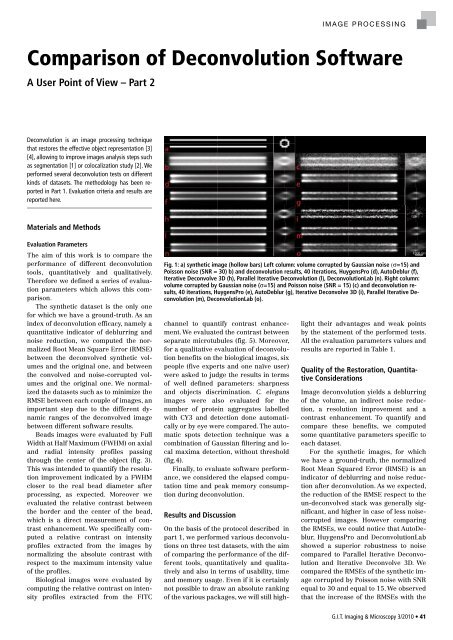
Fig. 1: a) synthetic image (hollow bars) Left column: volume corrupted by Gaussian noise (σ=15) and 

Poisson noise (SNR = 30) b) and deconvolution results, 40 iterations, HuygensPro (d), AutoDeblur (f), 

Iterative Deconvolve 3D (h), Parallel Iterative Deconvolution (l), DeconvolutionLab (n). Right column: 

volume corrupted by Gaussian noise (σ=15) and Poisson noise (SNR = 15) (c) and deconvolution results, 

40 iterations, HuygensPro (e), AutoDeblur (g), Iterative Deconvolve 3D (i), Parallel Iterative Deconvolution 

(m), DeconvolutionLab (o). 

channel to quantify contrast enhancement. 

We evaluated the contrast between 

separate microtubules (fig. 5). Moreover, 

for a qualitative evaluation of deconvolution 

benefits on the biological images, six 

people (five experts and one naïve user) 

were asked to judge the results in terms 

of well defined parameters: sharpness 

and objects discrimination. C. elegans 

images were also evaluated for the 

number of protein aggregates labelled 

with CY3 and detection done automatically 

or by eye were compared. The automatic 

spots detection technique was a 

combination of Gaussian filtering and local 

maxima detection, without threshold 

(fig.4). 

Finally, to evaluate software performance, 

we considered the elapsed computation 

time and peak memory consumption 

during deconvolution. 

Results and discussion 

On the basis of the protocol described in 

part 1, we performed various deconvolutions 

on three test datasets, with the aim 

of comparing the performance of the different 

tools, quantitatively and qualitatively 

and also in terms of usability, time 

and memory usage. Even if it is certainly 

not possible to draw an absolute ranking 

of the various packages, we will still highlight 

their advantages and weak points 

by the statement of the performed tests. 

All the evaluation parameters values and 

results are reported in Table 1. 

Quality of the restoration, quantitative 

considerations 

Image deconvolution yields a deblurring 

of the volume, an indirect noise reduction, 

a resolution improvement and a 

contrast enhancement. To quantify and 

compare these benefits, we computed 

some quantitative parameters specific to 

each dataset. 

For the synthetic images, for which 

we have a ground-truth, the normalized 

Root Mean Squared Error (RMSE) is an 

indicator of deblurring and noise reduction 

after deconvolution. As we expected, 

the reduction of the RMSE respect to the 

un-deconvolved stack was generally significant, 

and higher in case of less noisecorrupted 

images. However comparing 

the RMSEs, we could notice that AutoDeblur, 

HuygensPro and DeconvolutionLab 

showed a superior robustness to noise 

compared to Parallel Iterative Deconvolution 

and Iterative Deconvolve 3D. We 

compared the RMSEs of the synthetic image 

corrupted by Poisson noise with SNR 

equal to 30 and equal to 15. We observed 

that the increase of the RMSEs with the 

G.I.T. Imaging & Microscopy 3/2010 • 41

Image ProcessIng 

imaging-git.com/science 

image-processing 

Fig. 2: InSpeck green fluorescent 

bead, diameter 2.5 μm. Axial and 

transversal sections. Original image 

(a) and deconvolution results, 40 

iterations: HuygensPro (b), Autodeblur 

(c), deconvolutionLab (d). 

Fig. 3: Radial intensity profiles extracted from original and deconvolved 

images of an InSpeck green fluorescent bead, diameter 2.5 μm. 

HuygensPro and the DeconvolutionLab 

results, in the axial 

direction. To quantify the 

contrast enhancement, we 

computed the local relative 

contrast between the border 

and the center of the bead. In 

all the deconvolution results 

we pointed out contrast amelioration. 

This amelioration 

was particularly significant in 

AutoDeblur results. 

From the C. elegans images, 

FITC channel, we evaluated 

the contrast variation 

before and after deconvolution 

between adjacent microtubules 

(Figure 5). The contrast 

enhancement was 

particularly significant in AutoDeblur 

results. 

Quality of the Restoration, 

Qualitative considerations 

have been observed on HuygensPro 

results (see also fig. 

2). The outcomes from AutoDeblur 

and HuygensPro 

were nevertheless considered 

of high level and qualitatively 

equivalent. The results from 

DeconvolutionLab were generally 

judged fuzzier. 

Finally we compared the 

results of automatic and visual 

detection of spots on the C. 

elegans image, CY3 channel. 

On the non-deconvolved image 

the result of the automatic 

Fig. 4: detail from the result of 

deconvolution (HuygensPro, 40 

iterations) of c. elegans image, cY3 

channel. The green spots illustrate 

the result of the automatic detection 

of the protein aggregates. 

Number of spots recognized by 

eyes: 64. Results of automatic 

detection: not-deconvolved image 

90, HuygensPro result 61, Autodeblur 

result 84, deconvolutionLab 

result 65. 

detection was not reliable, as 

too many local maxima were 

detected. The numbers of 

spots detected on HuygensPro 

and DeconvolutionLab results 

were similar to the counting 

by a user (fig. 4). 

SNR decrease was much more 

significant for Parallel Iterative 

Deconvolution and Iterative 

Deconvolve 3D. Therefore 

these two tools appear less 

robust to noise. 

Concerning the bead acquisitions, 

we report the Full 

Width at Half Maximums 

(FWHMs) evaluated on intensity 

profiles extracted from 

the images before and after 

deconvolution. We always observed 

a reduction of the 

FWHMs in the results: after 

deconvolution the bead dimensions 

were closer to the 

original ones. This result 

shows how deconvolution improves 

resolution. The reduction 

of bead diameter in the 

deconvolved image was particularly 

consistent for the 

To evaluate the deconvolution 

results, we always started from 

a visual inspection of the data. 

Figure 1 depicts de-blurring 

and de-noise effects of 

deconvolution. We can observe 

that Parallel Iterative 


Deconvolve 3D give less good 

results compared to the other 

tools in case of highly noisy 

images. 

For a qualitative evaluation 

of the biological volumes 

restoration, six persons visually 

judged the deconvolution 

results. It emerged that the 

pushed contrast enhancement 

obtained with AutoDeblur 

can generate visually less 

realistic images, with more 

probable appearance of false 

structures. Strip-like artefacts 

Fig. 5: c. elegans embryo, FITc channel. Widefield image, Olympus cell R, 

100X 1.4NA oil objective. Voxel size 64.5 X 64.5 X 200 nm; dimensions 673 

X 714 X 111 pixels, 101 MB, 16 bit dynamic range. Transversal sections from 

the acquired image (a) and from deconvolution results with HuygensPro (b), 

Autodeblur (c) and deconvolutionLab (d), 40 iterations. For each image a 

particular is reported, together with the same intensity profiles evaluated 

throughout separate microtubules (note that for the intensity profiles 

absolute intensities are reported). 

42 • G.I.T. Imaging & Microscopy 3/2010

Image Processing 

Time and memory 

performance 

A final important consideration 

to be done concerns the 

performance of the tools in 

terms of runtime and memory 

consumption, as the deconvolution 

computational effort 

is in general particularly 

heavy. Parallel Iterative Deconvolution 

and Iterative Deconvolve 

3D open-source plugins 

are inferior in this sense. 

This is a considerable disadvantage, 

as the deconvolution 

can easily fail because of heap 

memory exception, even for 

images of common size. On 

our 10 GB machine we were 

not able to deconvolve the 

bead image, 32 MB, and the 

C. elegans image, 101 MB per 

channel, with these two plugins. 

As all the tests were performed 

on the same machine 

and in the same conditions, 

the processing time and the 

memory consumption of the 

different tools can be compared, 

numbers of iterations 

being equal. 

Conclusions 

The results of our tests are 

comparable as we followed a 

well defined working guideline 

(Part 1), and the same 

adequate effort was put into 

the optimization of deconvolution 

parameters for all the 

algorithms. 

All the tools that we considered 

showed good level 

performance in terms of results 

quality. With Parallel Iterative 


Deconvolve 3D we 

were not able to perform all 

the tests because of out-ofmemory 

exceptions. AutoDeblur 

showed a particularly high 

increment of contrast and 

produced much sharper results. 

This can facilitate the 

segmentation but makes the 

appearance of false structures 

more probable. HuygensPro 

produced results that 

appear more realistic to the 

expert eye, even if background 

artefacts were observed 

in the z direction. DeconvolutionLab 

showed a 

particularly good restoration 

of spatial resolution, but the 

results were generally con- 

Dataset Parameter Acquisition Huygens AutoDeblur Dec.Lab P.I.D. I.D.3D 

RMSE 

synthetic, SNR 30 5070 3010 2850 2880 2790 2620 

synthetic, SNR 15 6200 3030 2930 2940 4420 3370 

FWHM (in nm) 

bead radial 2867 2709 2709 2664 – – 

bead axial 4760 4000 4640 4160 – – 

Relative contrast (in %) 

bead 18 % 53 % 78 % 68 % – – 

C. elegans, FITC 15 % 33 % 50 % 28 % – – 

Qualitative evaluation (scale 1 to 5) 

C. elegans sharpness n. c. 3.2 4.2 2.0 – – 

C. elegans discrimination n. c. 3.6 4.3 2.2 – – 

Computation time (in s) 

synthetic, SNR 30 n. c. 66 143 33 992 1470 

bead n. c. 123 275 66 – – 

C. elegans, one channel n. c. 352 720 217 – – 

Memory consumption peak (in MB) 

synthetic n. c. 342 967 434 8821 2054 

bead n. c. 602 2439 734 – – 

C. elegans, one channel n. c. 1633 4811 1674 – – 

Deployment 

Installation/Usage n.c. Intuitive Intuitive 

License n.c. Commercial Commercial 

Platform n.c All Win All All All 

More 

expert 

Opensource 

More 

expert 

Opensource 

More 

expert 

Opensource 

Tab. 1: The values for the different evaluation parameters with regard to the different datasets are reported. In the 

‘Acquisition’ column the parameters values for the not-deconvolved images or for the simulated acquisition are 

reported. In the last five columns the parameters values for the deconvolution results with different software 

(HuygensPro, AutoDeblur, Deconvolution Lab (Dec.Lab), Parallel Iterative Deconvolution (P.I.D.) and Iterative Deconvolve 

3D (I.D.3D)) are reported. RMSE: normalized Root Mean Squared Errors between the synthetic image of six 

parallel hollow bars and the results of deconvolution with the different software. In the ‘acquisition’ column the 

RMSEs between the syntethic image and the same image blurred and corrupted by Gaussian and Poisson noise are 

reported. Radial and axial FWHM: in reference to the bead image, Full Widths Half Maximum evaluated on radial 

and axial profiles passing through the center of the object. Relative contrast: between the border and the center of 

the sphere for bead images and between separate microtubules for C. elegans images, FITC channel. Qualitative 

evaluation, scale from 1 (really bad) to 5 (really good); sharpness: capacity of well define objects shape by eyes; 

discrimination: capacity of distinguish close objects as separate. Runtime and memory consumption peaks. The 

squares with a dash indicate that it was not possible to complete the deconvolution because of out-of-memory 

exceptions. ‘n.c.’ means not computable. We indicated in bold types our favourite choice between software, for the 

different parameters and datasets. 

sidered fuzzier. DeconvolutionLab 

and HuygensPro 

showed better performances 

in terms of time and memory 

consumption. 

Both HuygensPro and AutoDeblur 

offer different possibilities 

for image pre-processing, 

such as background 

subtraction and spherical aberration 

corrections, which 

can certainly further improve 

the quality of the results but 

that were not applied in our 

tests to allow the comparison 

of the results. Moreover they 

are particularly user-friendly, 

especially concerning the setting 

of the deconvolution parameters. 

Parallel Iterative 


Deconvolve 3D are addressed 

to the more expert user as the 

parameter setting is less immediate. 

They do not implement 

pre-processing steps 

and are open-source software. 

Acknowledgements 

We thank our colleagues José 

Artacho, Thierry Laroche, 

J.-C. Floyd Sarria, Jane Kraehenbuehl 

and Virginie Früh 

(BIOp group) for their contribution 

and suggestions. We 

thank Debora Keller for C. elegans 

samples. We thank SVI 

and MediaCybernetics for 

their kind availability and for 

the demos of the software. 

References: 

For references, see Part 1. 

Authors: 

Alessandra Griffa, Nathalie Garin; 

BioImaging and Optics platform 

(BIOp), Ecole Polytechnique Fédérale 

de Lausanne (EPFL) 

Daniel Sage; Biomedical Imaging 

Group (BIG), Ecole Polytechnique 

Fédérale de Lausanne (EPFL) 

Contact: 

Nathalie Garin 

Leica Microsystems 

Heerbrugg, Switzerland 

nathalie.garin@leica-microsystems.com 

G.I.T. Imaging & Microscopy 3/2010 • 43

Comparison of Deconvolution Software - Biomedical Imaging Group ...

Create successful ePaper yourself

Delete template?

Save as template?