Mth229 - Department of Mathematics at CSI - CUNY

The College of Staten IslandDepartment of Mathematics10.80.60.40.20−0.2−25 −20 −15 −10 −5 0 5 10 15 20 25MTH 229Calculus I Computer Labhttp://www.math.csi.cuny.edu/matlab/MATLAB PROJECTSSTUDENT:SECTION:INSTRUCTOR:

BASIC FUNCTIONSElementary Mathematical functionsMATLAB notation Mathematical notation Meaning of the operation√sqrt(x)xsquare rootabs(x) |x| absolute valuesign(x) sign of x (+1, −1, or 0)exp(x) e x exponential functionlog(x) ln x natural logarithmlog10(x) log 10 x logarithm base 10sin(x) sin x sinecos(x) cos x cosinetan(x) tan x tangentasin(x) sin −1 x inverse sineacos(x) cos −1 x inverse cosineatan(x) tan −1 x inverse tangent

The College of Staten IslandDepartment of MathematicsMTH 229 Calculus Computer LaboratoryCourse OutlineThe main objective of this course is to reinforce calculus concepts and explore the applicationof calculus to solving problems by making use of a series of computer projects. The student willbe first introduced to mathematical software. In particular, MATLAB software will be used in thiscourse. MATLAB has capabilities for both numerical and symbolic calculations. It can also creategraphical output so that the results can be visualized more readily.The following projects are integrated with the material covered in courses MTH 230 CalculusI with Pre-Calculus and MTH231 Analytical Geometry and Calculus I. Therefore, full appreciationof these projects requires a solid understanding of the course material.1. Using MATLAB as a Calculator2. Plotting Graphs in MATLAB3. More on Graphing with MATLAB4. Graphical Solutions to Equations5. Investigating Limits in MATLAB6. Approximate First and Second Derivatives7. Critical and Inflection Points8. Newtons’ Method9. Optimization10. Definite Integrals and Riemann SumsExaminations: There will be a midterm and a final examination.Optional Materials:Software: MATLAB is installed in several of the campus computer labs. However, if you wishto work from home, you can purchase the MATLAB & Simulink Student Version R2007a at thestudent bookstore or online at http://www.mathworks.com/academiaOnline documentation can be found at http://www.mathworks.com/academia/student center

“Using MATLAB as a Calculator”MTH229The College of Staten IslandDepartment of MathematicsUsing MATLAB as a Calculator1 IntroductionThis project is designed to give you a brief introduction to the MATLAB software which will beused to help carry out your computer projects during this semester. This software is especiallydesigned for mathematical, scientific and engineering applications.Many of you probably have already used a scientific or graphics calculator like the TI-84. Inits simplest application, MATLAB can be used just like a graphing calculator. In this project welearn how to turn “math into MATLAB.” That is, we learn how to ask MATLAB math questionssuch as “what is 2+2?”1.1 New MATLAB topicsa. Arithmetic Operations and Precedence Rulesb. Function Evaluationc. Command Line Editor (correcting errors)d. Arrays and Tablese. Printing Textf. Resizing and Moving Windows1.2 New MATLAB commandsa. ; – The semicolon suppresses the output.b. x=a:h:b – This construct creates sequences of numbers.c. [x;y]’ – This construct creates a nice tabular look to lists of numbers.1.3 On-line resources for MATLAB and the MATLAB projectsThis project, and others, are available in an on-line format. Go to the following url for moreinformation:http://www.math.csi.cuny.edu/matlabhttp://www.math.csi.cuny.edu/matlab project 1 page 1

“Using MATLAB as a Calculator”1.4 Starting MATLABFigure 1: Initial MATLAB window contains Command Window, Workspace viewer, andCommand History panes.MATLAB is started by double clicking its desktop icon (on a typical installation of MATLABon Windows, other installations may vary). Figure 1 shows a typical startup window. It consists ofseveral panes. Additionally other windows, such as a help window or plot window, may appear.The visible panes in the figure are the Command Window which appears on the right side ofthe window. This window contains the command line where we type commands for MATLAB tointerpret. This will be our main method to interact with MATLAB. Additionally, in the upper leftpane is a Workspace viewer which shows the variables that are present in the MATLAB session,and in the lower left pane the Command History window displays the commands you have enteredinto the command window.Commands are typed after the prompt: >>. After they are typed in, the Enter key is hit to sendthe command to the MATLAB interpreter. MATLAB either shows the answer or will respond withan error message indicating why it couldn’t do what was requested.Multiple commands may be entered on the same line if the commands are separated by asemicolon ;, or a comma ,. As well, a semicolon at the end of a command causes its output not tobe displayed.http://www.math.csi.cuny.edu/matlab project 1 page 2

“Using MATLAB as a Calculator”2 Arithmetic OperationsWe begin our explorations with MATLAB by learning how to do simple arithmetic operations:For instance, adding 2 + 2 is done with>> 2 + 2ans =4After typing in the command (2 + 2), we typed the Enter key. MATLAB responded with ananswer of 4.Some other examples are shown below:symbol example MATLAB responseaddition + >> 3+4 ans = 7subtraction - >> 5 - 9 ans = -4multiplication * >> 5*9 ans = 45division / >> 8/9 ans = 0.8889exponentiation ^ >> 5^3 ans = 125The only symbol that may need learning is the ^ for powers.2.1 AssignmentWhen the command 2 + 2 is typed above, MATLAB evaluates it and responds with an answer of4. It then forgets about this calculation because we didn’t ask for it to be saved. In order to savevalues we can assign the output to a variable. After doing this, we can refer to the output by thevariable name.In the example below, we assign the value 18 to the variable a, the value 21 to the variable b,and the value 18 − 21 = −3 = a − b to the variable c.commandMATLAB response>> a = 18 a = 18>> b = 21 b = 21>> c = a - b c = -3Once a value is assigned to a variable, MATLAB remembers it until that variable is reassigned.Try predicting the responses to the following MATLAB commands to check your understanding.>> a = 3; b = 4;c = 5;>> a=b*cMATLAB responsehttp://www.math.csi.cuny.edu/matlab project 1 page 3

“Using MATLAB as a Calculator”>> b/a>> a=a-18>> a^bWhen you make an assignment, the variable name appears in the Workspace viewer whichappears in the upper left pane of the initial MATLAB window. You can view the contents of thevariable by double clicking it in the workspace viewer. Otherwise, you can enter just the variablename in the command line and its contents will be displayed.Exercise 1:a. What is the output of the following commands:>> a=3; b=4; c=5;>> a + b/c(1) Circle one:1. 3 4/52. 1.63. 3.84. 7/5Example 1:Assigning variables can simplify matters when used wisely. For example, when evaluating(2 − 3) − (−3).(−1) + 2One way is to write out the whole expression at once:>> ((2-3)-(-3))/((-1)+2)ans = 2There are many parentheses that are needed to get this right. This can make finding errors in ourwork tough. If we use spaces (which are ignored) and intermediate names, we can reduce thechance of a typing error:>> top = (2-3) - (-3);>> bottom = (-1) + 2;>> top/bottomans = 2This technique makes errors much easier to find.http://www.math.csi.cuny.edu/matlab project 1 page 4

“Using MATLAB as a Calculator”Exercise 2:a. Use assignment to help you compute3 − 32 − 2 · 32 · 3 − 2 .(2) Answer:3 Order of OperationsWhat is5 − 2/6?Is it 5 − 1/3 or 3 divided by 6? That is, 5 − (2/6) or (5 − 2)/6? We should know that thefirst is true because division happens before subtraction. What makes knowing this necessary isbecause there are two operations above, subtraction and division, and the answer will depend onwhich is done first. The order of operations act like a traffic cop directing the flow. MATLAB usesa fairly standard order of priority (precedence) for operations: addition and subtraction have thesame priority, which is below multiplication and division. Powers have the highest priority. Sotyping the command>> 5 - 2/6returns an answer of 4.6667 or 5 − 1/3, as division is done before the subtraction.In the following exercise you will review the basic order of operations.3.1 Multiplication/Division vs. Addition/SubtractionExercise 3:One of these things is not like the others. Which of these MATLAB commands is not like the othertwo? To help you out, try doing this with some values for a, b and c like>> a= 3; b=13; c= 23;a. (3) Circle one:1. >> a - b * c2. >> a - (b * c)3. >> (a - b) * chttp://www.math.csi.cuny.edu/matlab project 1 page 5

“Using MATLAB as a Calculator”b. (4) Circle one:1. >> a * (b - c)2. >> (a * b) - c3. >> a * b - cc. (5) Circle one:1. >> a / b + c2. >> a / (b + c)3. >> (a / b) + cd. (6) Circle one:1. >> (a + b) / c2. >> a + (b / c)3. >> a + b / ce. Which operations have higher precedence?(7) Circle one:1. multiplication/division2. addition/subtraction3.2 Multiplication/Division vs. ExponentiationExercise 4:Repeat the same exercise with the following expressions.a. (8) Circle one:1. >> a ^ (b * c)2. >> (a ^ b) * c3. >> a ^ b * cb. (9) Circle one:1. >> a * (b ^ c)2. >> a * b ^ c3. >> (a * b) ^ cc. (10) Circle one:1. >> a / b ^ c2. >> (a / b) ^ c3. >> a / (b ^ c)http://www.math.csi.cuny.edu/matlab project 1 page 6

“Using MATLAB as a Calculator”d. (11) Circle one:1. >> a ^ b / c2. >> (a ^ b) / c3. >> a ^ (b / c)e. Which operations have higher precedence?(12) Circle one:1. multiplication/division2. exponentiationf. Using the rules you found, evaluate the following expression and rewrite it with parenthesesshowing the order in which MATLAB evaluates the operations. (For example, a + b + c= (a + b) + c and not a + (b + c).) In this example there are 4 operations, so youranswer should have 3 pairs of parentheses.>> 7 - 3 ^ 2 / 9 + 4(13) Answer:3.3 Operations with the same precedenceHow does MATLAB interpret the following commands?>> 3 - 3 - 3>> 6 / 3 / 2>> 2 ^ 3 ^ 2There is an ambiguity as the answers are different if the leftmost operation is done first comparedto if the rightmost one is.http://www.math.csi.cuny.edu/matlab project 1 page 7

“Using MATLAB as a Calculator”Exercise 5:Evaluate the following expressions first using left-to-right order, and then from right-to-left. Enterboth answers separated by a comma.a. 3 − 3 − 3(14) Answer:b. 6/3/2(15) Answer:c. 2^3^2(16) Answer:Exercise 6:Investigate the expressions below to see the order in which the operations are performed by MAT-LAB. (For example, does 5 − 3 − 2 = (5 − 3) − 2 or 5 − (3 − 2)?)>> 5 - 7 - 8>> c - a + b - c>> 5 / 7 / 8>> 5 / 7 * 8 * 9What rule(s) does MATLAB use when evaluating expressions with two or more operations of thesame priority?(17) Circle one:1. from right to left2. from middle to end3. from left to rightExercise 7:Practice what you have just reviewed to evaluate the following. Let>> a=4;b=5;c=8;a.a b − c/bc − a(18) Answer:http://www.math.csi.cuny.edu/matlab project 1 page 8

“Using MATLAB as a Calculator”b.a (c−b)c − b(19) Answer:c.a 3/2b(20) Answer:d.a − b(c − a)c − a(21) Answer:Note: A full explanation of MATLAB’s priority rules is attached to this project in the ReferenceSection. You may want to review this to check your answers.3.3.1 Reusing previous commandsYou can save some typing if you learn how to reuse and edit your previously entered commands.The Command History window shows the commands you’ve typed during a MATLAB session.Double clicking on a command will paste it into the command window. The command history mayalso be accessed inside the command line by using either the up or down arrow to scroll throughyour previous commands.Once a command is at the >> prompt, you may make changes to it. Use the left or right arrowsto move around, or the mouse. Then you may insert text or delete existing text.Finally, you may type Enter to execute the new command. You do not need to have the cursorat the end of the line to do this.4 Function evaluationMATLAB allows much more than just the basic arithmetic operations. Extra functionality is providedby functions, such as sin, cos, or sqrt. A function is referred to by its name and used bycalling the function with its argument(s) enclosed in matching parentheses. A list of basic functionsand their MATLAB equivalents is attached to the end of the project in the Reference Section.For instance, the value of √ 15 is given by>> sqrt(15) # ans = 3.8730http://www.math.csi.cuny.edu/matlab project 1 page 9

“Using MATLAB as a Calculator”(The text after and including the number sign symbol is a comment and will be ignored if typedin.)Just typing the function name, without the parentheses, will show its definition.Here are a few more examples of function evaluations. Note that to get π = 3.1415 . . . , youtype pi; to get the number e = e 1 = 2.7182 . . . , you type exp(1).When trying these examples, if you get an error message, check that you have spelled thefunction name correctly. For example, if you type sqt(3) (you misspelled sqrt), MATLABresponds with the error message??? Undefined function or variable sqt.Try evaluating the following using MATLAB:MATLAB response>> sqrt(216) 14.6969>> pi pi = 3.1416... is built-in>> exp(1) ans = 2.7183 e is not built-in>> sin(pi/4) ans = 0.70711>> x = pi/3 x = 1.0472 assigns x>> tan(x) ans = 1.7321, as x = pi/3 by above>> sin(x)^2 + cos(x)^2 ans = 1, again, as x = pi/3Note: you will get better precision if you do not round off intermediate computations. Trytyping the following to see an example:>> pi/4>> sin(0.785)>> sin(pi/4)>> sqrt(2)/2When trigonometric functions are evaluated in MATLAB, arguments must be specified in radianmeasure—not in degrees. Recall, to convert from degrees to radian you multiply by π/180.Exercise 8:Use MATLAB to evaluate the following expressions.a. Calculate the sine of 40 degrees using MATLAB. MATLAB uses radians for all angle measurements.You will need to convert degrees to radians first.(26) Answer:b. Evaluate sin 2 65 ◦(27) Answer:c. Evaluate e (10−8.5)/3(28) Answer:http://www.math.csi.cuny.edu/matlab project 1 page 10

“Using MATLAB as a Calculator”d. Evaluate arcsin(sin(3π/4))(29) Circle one:1. 3π/42. −5π/43. π/45 VectorsWe will often want to apply a function to many different values of x. We’d like to do this in the mostconvenient manner. For example, to compute the function f(x) = x 2 cos 3 (x) for x = π/3, π/4and π/6 we can save some work by assigning a value to x and then computing:>> x=pi/3; x^2 * cos(x)^3>> x=pi/4; x^2 * cos(x)^3>> x=pi/6; x^2 * cos(x)^3This allows us to make a single change to x per line, instead of changing it in both places.Although the above technique is useful, there are better ways to do this task, as the MATLABlanguage is written to naturally apply the same function to many different values at once. In orderto do so we need to learn two things:a. How to store more than one number into a variable (vectors)b. How to apply a function to all the values of the vector simultaneously.5.1 Defining vectorsWe use the term vector to describe a MATLAB variable that contains lots of numbers at once.Vectors are made in MATLAB using the square brackets []. (MATLAB refers to vectors as arrays,a more general concept.)The simplest way to make a vector is to just type in the numbers you want inside of matching[]:(Don’t type the part with the % symbol. This is a comment to you.)>> x = [1,1,2,3,5,8,13,21] % start of Fibonacci sequence>> x = [1 1 2 3 5 8 13 21] % commas are optional>> somePrimes = [2,3,5,7,11,13,17,19,23]http://www.math.csi.cuny.edu/matlab project 1 page 11

“Using MATLAB as a Calculator”Exercise 9:Store the number 1, 2, 3 in a vector named x. Answer the following for this vector.a. What is x+x?(30) Circle one:1. The vector [1, 4, 9]2. The vector [2, 4, 6]3. An errorb. What is the output of x * x(31) Circle one:1. The vector [1, 4, 9]2. The vector [2, 4, 6]3. An error5.2 Arithmetic sequencesMany of the vectors of numbers we will deal with will be arithmetic sequences:a, a + h, a + 2h, a + 3h, . . . , a + kh = b, h > 0.We think of this in two ways:a. Numbers between a and b separated by a step size of hb. A certain number (k + 1) of numbers evenly spaced between a and b.There are two different ways in MATLAB to generate such sequences, depending on how youthink of the values in the sequence.5.2.1 numbers separated by a step size hTo generate a sequence of numbers separated by 1 is done using the : symbol, as in a:b:>> 1:5 % 1 2 3 4 5>> -1:5 % -1 0 1 2 3 4 5>> -(1:5) % -1 -2 -3 -4 -5The last example shows that the minus sign here means multiply each entry by −1.If we want a step size of h we use this syntax: a:h:b. For instance:>> evens = 0:2:10 % even numbers 0,2,4 ... 10>> evens = 0:2:9 % even numbers 0,2,4 ... 8. Stops at 8>> skip15 = 0:15:60 % 0,15,30,45,60 -- class is almost done>> skip15 = 15*(0:4) % same thing!>> skipafew = 1:98 % 1 2 skipafew 97 98http://www.math.csi.cuny.edu/matlab project 1 page 12

“Using MATLAB as a Calculator”Exercise 10:Find MATLAB commands which generate the following lists. Make sure your answer is correct.a. The odd numbers 1,3,...99(32) Answer:b. The numbers 10,20,30,...120(33) Answer:5.2.2 A fixed number of numbersWhen plotting functions we will desire a lot (say 100 or a 1000) of evenly-spaced numbers betweentwo points. Rather than figure out the step size between the points it is more convenient to specifyhow many linearly spaced points we want. This is done with the linspace function. Using it aslinspace(a,b) will produce 100 numbers between a and b. You can override the default of 100using a third argument:>> linspace(0,5,6) % ans = [0 1 2 3 4 5] (6 numbers)>> linspace(0,pi,3) % ans = [0, pi/2, pi] (3 numbers)Exercise 11:a. What linspace command produces this output:1.000 1.500 2.000 2.500 3.000 3.500 4.000(34) Circle one:1. linspace(1,7,4)2. linspace(1,4,1/2)3. linspace(1,4,7)4. linspace(1,1/2,4)b. What is the last value output by the command>> linspace(0,pi)(35) Answer:http://www.math.csi.cuny.edu/matlab project 1 page 13

“Using MATLAB as a Calculator”5.3 Applying arithmetic operations to vectorsIn MATLAB the basic object is a matrix (a rectangular collection of numbers). As such, the defaultdefinitions for +, -, ∗, /, and ˆ are the matrix definitions. What we will want is a little different.This means we will need to be careful when we multiply, divide or take powers of vectors.This will be discussed more in the next project. For this project, we focus on arithmetic operationswhich work as we would like: addition of vectors of the same size, and multiplication of avector times a number (a scalar).For example>> x = 1:5 % the numbers 1 2 3 4 5>> x + x % the numbers 2 4 6 8 10>> 3*x % the numbers 3 6 9 12 15>> 3*(x - 3) % subtract 3 then multiply:% -6 -3 0 3 6This allows us to do simple transformations, such as the conversion from Celsius to Fahrenheit,or back, given by these formulas:F = 9/5C + 32 or C = 5/9(F − 32)This is the basis of the last exercise.Exercise 12:Two common measures of temperature are the Fahrenheit and the Centigrade scales.a. Find room temperature in Celsius (F = 68 ◦ )(36) Answer:b. Find the average body temperature in Celsius (F = 98.6 ◦ )(37) Answer:c. Let X be a vector of Fahrenheit values between -100 and 100 in step size of 20, and Y bethe corresponding Celsius values. Which MATLAB commands give this?(38) Circle one:1. X=-100:10:100; Y=9/5*X+322. X=-100:20:100; Y=9/5*x+323. X=-100:10:100; Y=5/9*(X-32)4. X=-100:20:100; Y=5/9*(X-32)d. If two vectors are the same length, a table can be made from them that allows you to comparetheir entries. The syntax is either [X;Y] or [X;Y]’. Look carefully at the table of X and Yvalues. At what temperature is the Celsius and Fahrenheit measurement the same?(39) Answer:http://www.math.csi.cuny.edu/matlab project 1 page 14

“Using MATLAB as a Calculator”6 Reference Section6.1 Basic MATLAB commandsDescription Symbol(s) CommentsNumber (scalar) assignment a=7.25; b=1/12Scalar arithmetica+b; a-b; a*ba/b; a^bVector assignment x=a:h:b Fills array x with a, a + h, a + 2h, . . . , bx=[2 0 4 -7] Assigns sequence 2, 0, 4, −7 to xScalar/vector operations a*x, a+x If x = [3 0 -1] then 2*x = [6 0 -2]a-x, x/a x-2 = [1 -2 -3], etc.Careful: a/x and x^a won’t work.Pointwise vector operations a./x, x.^a If x = [3 0 -1], y=[8 2 2], thenx.*y, x./yx.^2=[9 0 1], x.*y=[24 0 -2], etc.The dot (.) makes it pointwise.Separator ; (semicolon) separates commands; suppresses outputseparates rows in a table or matrixTable [x;y] or [x;y]’ Two-row or two-column table6.2 Order of OperationsMATLAB uses the following symbols for arithmetic operations:Operation Symbol Precedence CommentExponentiation ^ 3 Highest precedenceMultiplication * 2Division / 2Addition + 1Subtraction - 1 Lowest precedenceIf an arithmetic expression contains nested parentheses, then the expressions contained withinthe innermost parentheses are evaluated first. In the absence of parentheses, the precedencerules decide the order of evaluation. The following rules apply:1. All operations with a higher precedence are carried out before those of lower precedences.Thus exponentiation is carried out first, then comes multiplication and division, and finally, additionand subtraction.2. If two operations have the same precedence then the operation on the left is carried out first.This is called the left-to-right scan rule.The examples in the following table show how the precedence rules help interpret arithmeticexpressions based on these rules. Try them out on the computer and make sure that you understandhow each expression is interpreted.http://www.math.csi.cuny.edu/matlab project 1 page 15

“Using MATLAB as a Calculator”Expression MATLAB value Interpreted as2*3+4*5 26 (2*3)+(4*5)2+3*4 14 2+(3*4)(2+3)*4 20 parentheses decides the order2/5*4 1.6 (2/5)*42/(5*4) 0.1 parentheses decides the order2^3^2 64 (2^3)^22^(3^2) 512 parentheses decides the order5/2/4 0.625 (5/2)/45/(2/4) 10 parentheses decides the order6.3 Basic FunctionsElementary Mathematical functionsMATLAB notation Mathematical notation Meaning of the operation√sqrt(x)xsquare rootabs(x) |x| absolute valuesign(x) sign of x (+1, −1, or 0)exp(x) e x exponential functionlog(x) ln x natural logarithmlog10(x) log 10 x logarithm base 10sin(x) sin x sinecos(x) cos x cosinetan(x) tan x tangentasin(x) sin −1 x inverse sineacos(x) cos −1 x inverse cosineatan(x) tan −1 x inverse tangentNOTE: MATLAB may give unexpected results when working with negative numbers, sinceits default is to assume inputs and outputs are complex numbers. Try evaluating sqrt(-4),(-8)^(1/3), and log(-5), to see what happens. Note that i represents √ −1.http://www.math.csi.cuny.edu/matlab project 1 page 16

“Plotting Graphs in MATLAB”MTH2291 IntroductionThe College of Staten IslandDepartment of MathematicsPlotting Graphs in MATLABMathematically, a function f is a rule that assigns to each value x in its domain, a correspondingvalue of y in its range. The graph of a function is then the collection of all points (x, y) such thaty = f(x), sketched in the Cartesian plane. Of course we can’t realistically expect to draw the(typically) infinite collection of points. In a calculus class we learn to sketch graphs by focusingon their important features: zeroes, asymptotes, limits, points of discontinuity or non-smoothness,relative maxima and minima, and points of inflection. With these important features understood, asketch then can be drawn accurately where need be and filled in broadly otherwise.With MATLAB we take a different approach. To plot the function f over the interval [a, b],we actually plot as many pairs of points (x, y) as necessary to ensure an accurate representation ofthe graph. How many points? There are no good rules. We’ll see examples (lines) where two areenough. As well, we will see examples where we can’t possibly take enough points to do what wewant. We’ll just have to get used to experimenting to find the correct amount.With this approach, we need to be able to do the following:a. generate the x values of the points in our graph,b. generate the corresponding y values,c. plot the points and connect them with lines.We’ve seen how to make regularly spaced x values using either the a:h:b construction or thelinspace function. In this project we’ll learn how to make the corresponding y values, and howto then make the desired plot.1.1 New MATLAB topics• Vector mathematics and the dot symbol• Graphing functions using pairs of vectors• Exploring a graph with the command line and the mouse• Annotating a graph• Printing a graphhttp://www.math.csi.cuny.edu/matlab project 2 page 1

“Plotting Graphs in MATLAB”1.2 New MATLAB commands• a:h:b, linspace(a,b,n) – used to generate regularly spaced sequences of points.• The dot operators: ’.*’, ’./’, ’.^’. – used in vector mathematics.• plot(x,y) – plot the two lists of numbers2 Graphing with MATLABThink back to how you first learned to graph a function or an equation. What would you do if youwanted to plot a graph of the parabola y = x 2 over the interval −2 ≤ x ≤ 2? We could choose aset of x values, say, x = −2, −1, 0, 1, 2, then square each x value to determine the correspondingy value (y = 4, 1, 0, 1, 4). These might be displayed together, as in the following table:x -2 -1 0 1 2y 4 1 0 1 4We would then mark each corresponding (x, y) pair as a point on a Cartesian coordinate system,and connect the points with straight lines.Example 1:To graph f(x) = x 2 over the interval [−2, 2] using MATLAB we just need to know that the plotfunction will make the desired plot. Then we have (the % and beyond are comments and need notbe typed in.)>> x = [-2 -1 0 1 2] % creates the vector x=[-2 -1 0 1 2]>> y = [ 4 1 0 1 4] % creates the y values>> [x;y] % display as a tableans =-2 -1 0 1 24 1 0 1 4>> plot(x,y) % plot points and lineshttp://www.math.csi.cuny.edu/matlab project 2 page 2

“Plotting Graphs in MATLAB”43.532.5(−2,4)x = [−2 −1 0 1 2]y = [ 4 1 0 1 4](2,4)21.5(−1,1) (1,1)1(0,0)0.50−2 −1.5 −1 −0.5 0 0.5 1 1.5 2Figure 1: The function f(x) = x 2 plotted with 5 points.Figure 1 shows that our graph isn’t quite what we expected. Rather than looking like a familiarparabola, we see a sequence of straight lines. How can we fix that? By taking more points.We have an easy way of taking more points, we can generate a 100 of them with the commandlinspace(-2,2) and, if need be, 1,000 with the command linspace(-2,2,1000). However,we don’t want to do all the squaring by hand. Rather MATLAB should do the work. The nextexample shows how to do this for f(x) = x 2 , and later on in this project we’ll see how to do thisfor other functions.>> x= linspace(-2, 2)>> y=x.^2; % notice the ".^" and not just "^">> plot(x,y) % makes the plot43.532.521.510.50−2 −1.5 −1 −0.5 0 0.5 1 1.5 2Figure 2: The function f(x) = x 2 plotted using 100 points.Using more points requires no more labor on your part than using just 5 points. If we didn’thave enough we’d take more and replot. However, our graph (in Figure 2) now looks okay. Eventhough it may no longer be evident, the graph still consists of a sequence of straight lines!http://www.math.csi.cuny.edu/matlab project 2 page 3

“Plotting Graphs in MATLAB”We repeat the previous example with a different function.Example 2:Graph the function f(x) = e x over the interval [−1, 1].We’ll need to know that in MATLAB the function exp(x) performs e x . Other than that, thisexample follows the three steps in plotting:a. We want to plot the function over the interval [−1, 1]. To do so, we first choose evenly spacedpoints between −1 and 1 with a step size of 0.5>> x = -1:0.5:1 % no ’;’ means you see all the valuesb. We then define the y values for each x value using exp:>> y = exp(x) % again you see all the values as no ’;’c. Finally we use plot( ) to view the function’s graph:>> plot(x,y) % does your answer match the graph shown?32.521.510.50−1 −0.8 −0.6 −0.4 −0.2 0 0.2 0.4 0.6 0.8 1Figure 3: The function f(x) = e x plotted with 5 points.As shown in Figure 3, this graph created with 5 sample points in [−1, 1] is obviously not sosmooth. To obtain a smooth looking curve one needs to define more x points. The exact numbervaries depending on how rapidly the function varies over its domain. We start with the simpledefault of 100 using linspace and see if this is enough:>> x = linspace(-1,1)>> y = exp(x)>> plot(x,y)>> grid % add a grid to the graphhttp://www.math.csi.cuny.edu/matlab project 2 page 4

“Plotting Graphs in MATLAB”32.521.510.50−1 −0.8 −0.6 −0.4 −0.2 0 0.2 0.4 0.6 0.8 1Figure 4: The function f(x) = e x plotted with 100 points.The graph in Figure 4 shows that 100 points is sufficient to present a smooth looking curve.It is important that even though only the line defining the values for x is different, you mustagain evaluate the second and third lines. The values stored in y do not update automatically. Ifyou forgot to recreate the y values, you would be trying to pair off the 100 x values with only 5 yvalues and an error would occur. For such a simple function we can avoid this step by defining ywithin the plot function, as in>> plot(x, exp(x))Exercise 1:Create a graph of y = cos 4x over [0, π]. To illustrate what happens when there are too few pointsin your domain, first try a step size of π/10 (pi/10).a. Which command gives the desired values for x?(1) Circle one:1. x=0:pi/10:pi2. x=0:pi:pi/103. x=linspace(0,pi)http://www.math.csi.cuny.edu/matlab project 2 page 5

“Plotting Graphs in MATLAB”b. Which command gives the correct answer for y?(2) Circle one:1. y = cos(4x)2. y = cos4*x3. y = cos(4*x)c. Plot your graph with the plot command. You don’t need to turn it in.d. Redo your plot, this time using the command >>x=linspace(0,pi) to define the x array.Which plot looks more like the plot of a cosine curve?(3) Circle one:1. The first one2. the second one3. both of themExercise 2:We wish to plot the function f(x) = e cos(x) over the interval [0, 2π].a. What command generates a sufficient number of values for x?(4) Circle one:1. linspace(0,2*pi)2. linspace(0,100,2*pi)3. 0:2*pi4. 0:2*pi:0.01b. Which command will generate the corresponding y values:(5) Circle one:1. exp^cos(x)2. e^cos(x)3. exp(cos(x))4. exp(x)cos(x)3 Algebraic expressions with vectorsWe now know pretty well how to create the values for x using linspace or a:h:b. To create thevalues of y is a little harder. We want to create the values simultaneously and so must use theproper MATLAB syntax.http://www.math.csi.cuny.edu/matlab project 2 page 6

“Plotting Graphs in MATLAB”For concreteness we call a single number a scalar and a set of numbers a vector. (AlthoughMATLAB thinks of them both as examples of arrays.)Suppose we have two terms a and b and want to find one of these arithmetic operations: a+b,a-b, a*b, a/b, or a^b. The answer depends on the whether the terms are scalars or vectors:If both a and b are scalars Then no special care is needed.If one of a or b is a vector When one of the terms is a scalar and the other a vector then twocases won’t work as expected. First with powers, a ^ b, involving a vector, You will needto use the notation .^ in place of ^. This is why we used x.^2 in our first example, insteadof simply x^2. Second, when dividing by a vector you need to use the notation ./ and notsimple /. These extra “dot’s” are important to learn.If both a and b are vectors When both terms are vectors and both have the same length,then a*b, a/b, and a^b need to use a “dot,” as ina .* b, a ./ b, a .^ b(In fact, you could always use the dot form in the other instances, but it is not required, and looksreally bad.)Example 3:Let’s see what happens if you don’t know how to work with arrays. We define x to be the numbers1 through 5:>> x = 1:5x = 1 2 3 4 5We might try to multiply x by 10.>> 10*xans = 10 20 30 40 50Which does what we expected. What about dividing by 10?>> x/10ans = 0.10000 0.20000 0.30000 0.40000 0.50000What about adding 10?>> x + 10ans = 11 12 13 14 15So what’s the fuss? Well we’ve been lucky. Try to divide x into 10:>> 10/xERROR, ERROR WILL ROGERS.http://www.math.csi.cuny.edu/matlab project 2 page 7

“Plotting Graphs in MATLAB”How about squaring x:>> x^2ERROR, ERROR WILL ROGERS. I’M BEGINNING TO SMOKE!How about trying to multiply x by itself>> x*xERROR, ERROR WILL ROGERS. I CAN’T TAKE IT ANYMORE. READ THE MANUAL.Actually, the error messages say something like the first one:??? Error using ==> /Matrix dimensions must agree.For 10/x, MATLAB is trying to use matrix division which is not defined for this problem. Wewant our division to be element by element, so we need to specify the extra “dot.”Go back and check that>> 10 ./ x>> x .^ 2>> x .* xwork as expected.Here are some examples where the vector notation is used:Example 4:Plot y = sin x + cos 3x over the domain [0, 2π].>> x = linspace(0,2*pi);>> y = sin(x)+cos(3*x);>> plot(x,y)We didn’t need any dots as 3*x is a scalar times an vector, The sin and cos functions are smartabout vectors, and the + is between two vectors of the same size.Example 5:Plot y = e −x/2 cos 6x over the domain [0, 10π]:>> x = linspace(0,10*pi);>> y1 = exp(-x/2); % no dot for -x/2 since 2 is a scalar>> y2 = cos(6*x); % Break up the computation into bite-sized pieces>> y = y1.*y2; % dot needed since y1 and y2 are both vectors>> plot(x,y)http://www.math.csi.cuny.edu/matlab project 2 page 8

“Plotting Graphs in MATLAB”Again the dot . before the * means that multiplication of the two same-sized vectors y1 and y2is to be carried out element-by-element. To minimize the chance of errors, we broke the probleminto intermediate calculations by using two variables y1 and y2.Example 6:Plot y = 1/(x 2 − 1) over the domain [2,5]:>> x = 2 : 0.1 : 5;>> y = 1./(x.^2-1);>> plot(x,y)Here the “dot” is used twice—powers (x 2 ) always get a dot when a vector is involved, and thedivision by a vector requires the extra dot.Exercise 3:Define a, b and c by>> a = 1:2:20; b = 1:10; c = 1:2:10;Which of the following is defined?a. b+c(6) Circle one:1. yes 2. nob. a + b(7) Circle one:1. yes 2. noc. a./ b(8) Circle one:1. yes 2. nod. a * b(9) Circle one:1. yes 2. nohttp://www.math.csi.cuny.edu/matlab project 2 page 9

“Plotting Graphs in MATLAB”Exercise 4:Let x=[1 2 3]. Translate the following math statements into MATLAB commands. To help, thevalue for the function when x=[1 2 3] is given in parentheses.a. Write MATLAB commands to compute:cos(x) sin(x)ans =0.4546 -0.3784 -0.1397(10)b. Write MATLAB commands to compute:sin(x) 2ans =0.7081 0.8268 0.0199(11)c. Write MATLAB commands to compute:sin(x 2 )ans =0.8415 -0.7568 0.4121(12)http://www.math.csi.cuny.edu/matlab project 2 page 10

“Plotting Graphs in MATLAB”d. Write MATLAB commands to compute:f(x) = 7x 2 sin( 17x 2 )ans =0.9966 0.9998 1.0000(13)e. Write MATLAB commands to compute:ans =(14)f(x) = x −cos(x) − sin(x)sin(x) + cos(x)1.2180 4.6877 1.6675f. Write MATLAB commands to compute:ans =(15)f(x) = 1 x3/2(x −10 10 )20.0810 0.2949 0.6152http://www.math.csi.cuny.edu/matlab project 2 page 11

“Plotting Graphs in MATLAB”3.1 How to submit graphsIf you turn your work in on paper, you may be asked to print out a graph and attach it to yourproject. Printing a graph can be done using the printer icon or Print... dialog under the Filemenu of the figure window.If you submit your work through the web interface, you must attach your graph to your projectwhen you save or submit your work. This is done with the following steps:a. First save your graph as a JPEG file using the Save As... under the File dialog of thefigure window (Figure 5). If you name your file with a .jpg extension, MATLAB will savethe figure in this format. You should save the figure in your My Documents directory, yourdesktop, or some other place that is easy to find.b. You then attach the saved jpeg image using the browse button in the web form. When theproject is saved or submitted your image file(s) will also be included. You can verify what issaved by clicking the new link accompanying the question.You do not need to do this each time you save the project, the files are stored on the server.They can be overwritten if a new file is attached.Figure 5: To save graphs to attach to project for web submission, use the Save As... dialogunder the File menu.http://www.math.csi.cuny.edu/matlab project 2 page 12

“Plotting Graphs in MATLAB”Exercise 5:Graph the function f(x) = sin((π/2)x) + sin((2/5)πx) over the interval [0, 40].a. How many peaks (relative maxima) does the graph have?(16) Answer:b. This function is periodic. How many periods are graphed in [0, 40]?(17) Circle one:1. 22. 33. 44. 55. none of the abovec. Estimate from your graph the value of f(10) to at least 1 decimal point.(18) Answer:d. Upload your graph.(19) Attach your graph to the worksheet.Exercise 6:a. Graph the function f(x) = cos 2 (x) − sin 2 (x) over the interval [−2π, 2π]. Use 100 points inthe domain.(20) Attach your graph to the worksheet.b. Does the graph resemble any graph that you are familiar with?(21) Circle one:1. cos 2x2. cos x/23. cos xhttp://www.math.csi.cuny.edu/matlab project 2 page 13

“Plotting Graphs in MATLAB”Exercise 7:For this exercise we look at the graph of the polynomial function f(x) = x 3 − 20x 2 + 10x − 1.a. First plot the function over the interval [−10, 10]. What is the approximate range for they-axis?(22) circle one:1. [-10,10]2. (-10,10)3. [-3100,0]4. [0, 2π]b. We wish to investigate when (if) this function is positive. We can’t readily tell from ourgraph so we will replot over a smaller domain. Which of these domains seems appropriatefor this task?(23) circle one:1. [0,500]2. [0,10]3. [-1,1]4. [0, 2π]c. Replot the graph over the selected domain. Turn on the grid by entering the command>> gridFrom your graph, which of these x values have f(x) > 0?(24) Circle all that apply:1. 02. 0.253. 0.504. 0.75http://www.math.csi.cuny.edu/matlab project 2 page 14

“More on Graphing with MATLAB”MTH2291 IntroductionThe College of Staten IslandDepartment of MathematicsMore on Graphing with MATLABWe’ve seen that basic plots may be produced in MATLAB by following three steps: produce anappropriate selection of x values; generate the corresponding y = f(x) values; plot the two vectorswith the command plot(x,y).In this project we show how to handle various situations that arise when plotting functions thatrequire us to think before we start making our plots. These include: figuring out an appropriatedomain for the plot; plotting functions with vertical asymptotes; plotting more than one functionon the same graph; and plotting functions which are defined differently over different intervals.Additionally, we learn how to add color, labels, and titles to a figure.1.1 New MATLAB Topicsa. Plotting Several Functions on the Same Graphb. Plotting Functions Defined by Several Equationsc. Exploring Graphs with the Moused. Annotating Graphs1.2 New MATLAB Commandsa. zoom [on off] – use the mouse to ’zoom’ in on parts of the graph.b. plot(x1,y1,x2,y2) – plot multiple graphs at once.c. hold [on off] – hold the current graph.2 Using zoom to explore a figureOnce a function is plotted, we typically want to use the figure to answer questions about the function.Example questions are: When does the function equal 0? When is the function at its lowestpoint? Where is the function increasing? These can be answered by focusing on one or two pointson the graph. To read the values of these points we can use the label on the x and y axes. However,to get more precise answers it is useful to be able to “zoom” in on the graph to narrow the range ofhttp://www.math.csi.cuny.edu/matlab project 3 page 1

“More on Graphing with MATLAB”the axes. This can be done by replotting the function over a smaller domain. This is recommendedif you want the most accuracy. However, the zoom function allows us to quickly (if not roughly)identify these points of interest.The zoom feature may be turned on by entering the command >> zoom on and turned off byentering the command >> zoom off. Alternately, on the figure window are two icons for settingthe zoom features. These are shown in Figure 1.Figure 1: Icons in graph window to adjust zoomClicking the + magnifying glass allows you to zoom into a figure. When you click the mouseanywhere in the figure, the figure will be replotted using 1/2 of each axis; in effect, you zoom inby a power of 4. If you want more than this, you can use the mouse to drag out a box on the figure.When the mouse button is released the highlighted window area is shown. The - magnifying glassreverses the zoom style.Exercise 1:To illustrate, type in the following commands, which plot the function f(x) = sin(x 2 ) over theinterval [0, π].>> x = linspace(0, pi);>> y = sin(x.^2);>> plot(x,y); grid>> zoom on % just zoom works here tooNow clicking in the figure window will cause the graph to be redrawn over a smaller domain.a. Click near the smallest positive x in this interval where f(x)=0. (The positive x-value wherethe graph first crosses the x axis). What is the length of the interval shown on the y axis?(1) Answer:b. Click twice more near this point of first intersection. Estimate (no more than two decimalpoints) from the zoomed in graph the numeric value of the x for which f(x) = 0.(2) Answer:c. Click the - magnifying glass and zoom out. Then the + magnifying glass to zoom in. Thistime on the second intersection point. Click near it 3 times. Estimate this value of x forwhich f(x) = 0.(3) Answer:http://www.math.csi.cuny.edu/matlab project 3 page 2

“More on Graphing with MATLAB”3 Identifying an appropriate domainMATLAB can’t think for us, but it can help us “think easier.” Case in point, we’re often interestedin plotting a function on only part of its domain. This may be where a function makes sense fora physical problem such as non-negative time, or non-negative area. Or, it may be where we canidentify one cycle of a periodic function. We can analyze the function to do this, or we can useMATLAB to explore some graphs and from these decide upon an appropriate domain.Example 1:A baseball is thrown from center field towards home plate. Its height, y, varies as a function oftime, t. It is known from high-school physics that a model for this is given by the projectile motionformulay = y 0 + v 0 t − 1 2 at2 ,where y 0 and v 0 are the initial height and upward velocity, and a is the constant of acceleration. Inmetric units of meters and seconds, we will assume a = 10 instead of the more accurate 9.8 m/s 2 .Suppose a ball is thrown with an initial velocity of v 0 = 10 meters per second upward from aninitial height of y 0 = 2 meters. On what realistic domain will y(t) ≥ 0?Mathematically, y(t) is a parabola which opens downward as the t 2 coefficient is negative. Wecould use formulas to find a parabola’s zeroes, but using MATLAB we can have fun exploring thegraph just as easily. First, we make an initial plot of the data over the interval [0, 10]. Why that?Well time must be non-negative so t ≥ 0 is natural. As for 10, since this is supposed to model aball being thrown, 10 seconds should be long enough, if the model is realistic.>> t = linspace(0,10);>> y = 2 + 10*t - (1/2)*10*t.^2;>> plot(t,y)If you make this graph, you’ll see that 10 seconds was too long. (Why). Let’s replot using aninterval of [0, 2].>> t = linspace(0,2);>> plot(t,2 + 10*t - (1/2)*10*t.^2)(We combined the definition of y directly into the plot function.)Now our interval is too small.Exercise 2:Replot the ball problem until you can find a good estimate for the value of b so that y(t) ≥ 0 onthe interval [0, b], and is negative for t > b. What is the value of b that you found?(4) Answer:http://www.math.csi.cuny.edu/matlab project 3 page 3

“More on Graphing with MATLAB”Example 2:Now suppose we want to plot one period of this periodic sine function:f(x) = 50 + 30 sin( 2πx365 )We could try to remember the rules for the shape of sine curves based on the general formaty = d + sin(bx + c). This is best, but do you remember? What we can do without having toremember is to plot this formula over a few different viewing windows until we can figure it out.Here is an example with comments53.5Too small80Not enough537552.55251.55170656050.555500 2 4 6 8500 20 40 60 80 10080Too much80Just right!70706060505040403030200 200 400 600 800 1000200 100 200 300 400Figure 2: Different viewing windows to frame one period of a sine function.>> x=linspace(0,2*pi); plot(x,50+30*sin(2*pi*x/365))%% [0,2pi] is always a good start, but it is too small. Try a larger domain>> x=linspace(0,100); plot(x,50+30*sin(2*pi*x/365))%% Still too small. Be bold let’s see try 1000>> x=linspace(0,1000); plot(x,50+30*sin(2*pi*x/365))%% Oops, too big now>> x=linspace(0,365); plot(x,50+30*sin(2*pi*x/365))%% just right. Oh yeah T=(2*pi/b)!That doesn’t take too long, as we only need to change one number and rerun the line. To takeadvantage of the “up arrow” trick, we put the commands on one line and combined the functionevaluation with the plot function.http://www.math.csi.cuny.edu/matlab project 3 page 4

“More on Graphing with MATLAB”Exercise 3:Find the suggested values by plotting the graphs until you can figure out the answer.a. Repeating the above example, find one period of the functionf(x) = 120 sin(120πx).(This is a bit tricky! Keep plotting until you clearly get one period shown in the viewingwindow.)(5) Answer:b. When does f(x) = 25 − x − sin(x) cross the x-axis? (Guess an answer to within 1 decimalpoint.)(6) Answer:4 Plotting functions with vertical asymptotesPlotting functions with vertical asymptotes can cause troubles. For instance, suppose we want toplot the function f(x) = 1/ sin(x) over the interval [0, π]. A first attempt may look like this:>> x = linspace(0,pi);>> plot(x, 1./sin(x))If you make this graph, you’ll find that it doesn’t look like what you would expect. In this casethe function has a vertical asymptote at both endpoints 0 and π. This means that when the x valuesare close to the endpoints, the corresponding y values get to be very large. This is why the y-axisis labeled using scientific notation indicating 15 zeroes after the numbers. This makes this graphworthless for answering questions about f(x). The remedy is to replot, only this time avoiding theasymptotes:>> delta = 0.1>> x = linspace(delta, pi-delta)>> plot(x, 1./sin(x))This is much better, allowing us to see the shape of the graph. We used a variable delta sothat if we wanted to, it is easy to make changes.Exercise 4:From its graph, estimate the minimum value of the functionf(x) = 5cos(x) + 8sin(x)over the interval (0, π/2).Just plotting with x values given byhttp://www.math.csi.cuny.edu/matlab project 3 page 5

“More on Graphing with MATLAB”>> x = linspace(0,pi/2)will cause the same problems as above. Make a plot, judiciously avoiding the vertical asymptotes,and then find the minimum value (y value) of the function on this interval.(7) Answer:Exercise 5:Although it isn’t an asymptote, this next problem has the same problem with the default y-axisscale being too big to accurately see other features of the graph.Letf(x) = x 5 − 225x 3 − x 2 + 225.Our goal is to find the three real roots (zeroes) of this polynomial.a. First plot the graph on the interval (−17, 17). What are the values of the x intercepts thatyou can clearly see.(8) Answer:b. Is 0 the other root? From the graph over −17, 17 it seems plausible. Explain why you knowthat 0 is not the other real root for this polynomial.(9) Answer:c. Replot the function over an appropriate domain to find the third real root:(10) Answer:5 Plotting Several Functions on the Same GraphOften we wish to compare two functions. We may want to see which is bigger? Which growsfaster? Or, we may want to see when they are equal. In order to do this we need to learn how toput multiple graphs into one figure. We illustrate two ways that this can be done:a. You can draw all the graphs at once using plot, as in plot(x1,y1,x2,y2).b. You can use the hold function to cause MATLAB not to draw a new plot each time, butrather to hold the current plot so that new lines may be added to it.http://www.math.csi.cuny.edu/matlab project 3 page 6

“More on Graphing with MATLAB”Example 3:Plot the functions f(x) = 4 cos x and g(x) = cos 4x together over the interval 0 ≤ x ≤ 2π.Solution: We first create pairs of arrays as if we were to graph each function separately.>> x = linspace(0,2*pi);>> y1=4*cos(x); % this is the first function>> y2=cos(4*x); % the second function needs a different name>> plot(x,y1,x,y2), grid % plot(x,y) is one graph. This makes twoMATLAB creates a frame in which all function values fit, and then plots the graph of eachfunction. Different colors are used for each function.If we prefer, plot(x,y1,x,y2) can be replaced with:>> plot(x,y1)>> hold on % next plot will be on top of the current one>> plot(x,y2)>> hold off % turn off the hold. Next graph opens a new windowThe hold on command instructs MATLAB not to create a new plot window with subsequentplot calls. By entering hold off at the end of the example, we allow new plot windows to becreated.Exercise 6:Consider the functions of the previous example, y 1 = 4 cos (x) and y 2 = cos (4x), make the graphsand use them to answer the following:a. Which function is oscillating more rapidly?(11) Circle one:1. cos(4x)2. 4 cos(x)b. Which function has the larger amplitude?(12) Circle one:1. cos(4x)2. 4 cos(x)http://www.math.csi.cuny.edu/matlab project 3 page 7

“More on Graphing with MATLAB”Exercise 7:Let f(x) = √ x. Plot f(x) and g(x) = f(x) − 5 together over the interval [0, 10]. The graph ofg(x) is the graph of f(x) shifted ...(13) Circle one:1. left by 52. down by 53. right by 54. up by 5Exercise 8:We wish to graph a function and its tangent line. Graph both the function y = √ x over the interval[0, 9] and the line through the point (4, 2) with slope 1/4.(14) Attach your graph to the worksheet.5.1 Plotting Functions Defined by Several EquationsExample 4:Cell phone plans often have a flat rate for a fixed amount of minutes and then a per minutecharge for each minute over the fixed amount. Mathematically, this is described by a function withtwo different definitions depending on which part of the domain – if the value is less than the fixedamount or more.For instance, if a company offers 500 minutes of calling for $25 and thereafter it is 25 centsper minute, a function that describes the amount you owe based on the number of minutes is{ 25 if 0 < x ≤ 500f(x) =25 + .25(x − 500) if 500 < x(Neglecting the onerous extra charges and taxes of course.)To plot this function (Figure 3), we handle each part of the function definition separately.>> x1 = linspace(0,500);>> y1 = 25 + 0*x1; % note the funny 0*x1>> x2 = linspace(500,1000);>> y2 = 25+.25*(x2-500); % if x>500 we use this line>> plot(x1,y1,x2,y2),grid % plot bothThis example shows a funny trick to plot the horizontal line y2 = 25+0*x1 instead of simplyy2 = 25. Try plotting both ways to see why we did so.http://www.math.csi.cuny.edu/matlab project 3 page 8

“More on Graphing with MATLAB”160But is the long distance free?14012010080slope = .256040$25 fior first 500 minutes200 100 200 300 400 500 600 700 800 900 1000Figure 3: Plot of phone chargesExercise 9:Plot a graph that describes the following calling plan: You pay $35 for the first 1,000 minutes.After the first 1,000 minutes you pay $0.30 per minute. Draw a graph for usage between 0 and2,000 minutes.a. What commands did you use?(15)b. (16) Attach your graph to the worksheet.6 Adding additional information to a graphicWe may want to add additional information to a graphic. This may be done when we issue a plotcommand, or through the dialogs offered by the figure window.Here are few things that you can do:Setting a plot to have a certain color When you plot two vectors you can set the color ofthe line that is drawn by adding it as a third argument, such ashttp://www.math.csi.cuny.edu/matlab project 3 page 9

“More on Graphing with MATLAB”>> plot(x,y,’g’) % ’g’ for green.Some other basic colors are ’b’ for blue, ’r’ for red, ’y’ for yellow.Plotting points, not line segments You can plot the two vectors as just points by specifyingthe type of point you want drawn, as the color is specified above. For instance>> plot(x,y,’.’) % plots with dots, doesn’t connect lineOther characters are ’o’ for circles, ’+’ for plus signs, ’x’ for crosses, ’d’ for diamonds,and ’s’ for squares.Adding text to a figure Check the Figure Pallette dialog under the View menu. You mayhave to maximize the figure window. You will see, as in Figure 4, a variety of items forannotating your graph. You can label your functions by adding text with an arrow. Try thetext arrow dialog. Just point, ’drag-and-drop’, then type your text. Alternately, use thegtext command from the Command Prompt. (Type help gtext for usage.)Figure 4: Figure Pallette menu for adding text, arrows and lines to a figure.Labeling the axes The Axes Properties dialog under the Edit menu in the figure windowallows you to add a title, and edit your axis labels, among other things.http://www.math.csi.cuny.edu/matlab project 3 page 10

clinical trial. Using noninformative priors and success rates of the 2 interventions in the 2 trials, wegenerated the posterior distribution of the difference in success rates. From the posterior distribution, wecomputed the probabilities that the success rate of ADR was better than the success rate of spinal fusion.In addition, using 2 noninferiority margins of -10% and -15%, we computed the probabilities that thesuccess rate of ADR was not inferior to the success rate of fusion. Finally, using the posterior distributionwe computed the same probabilities for a new trial (Prediction).ResultsThe sensitivity analyses revealed that the influence of missing data on the outcome measure of clinicalsuccess was minimal.The Bayesian model that used data on completers indicated that the probability for ADR being better thanspinal fusion was 79% (Table 17). The probability of ADR being noninferior to spinal fusion using a -10% noninferiority bound was 92%; using a -15% noninferiority bound, it was 94%. The probability ofartificial discs being superior to spinal fusion in a future trial was 73%.Table 17: Results of Bayesian Model Analyses*SR[d] – SR[f](d; 95% CR)†P: d > 0, % P: d > -0.10, % P: d > -0.15, %Blumenthal 2005 0.07(-0.013–0.19)91 99 100ProDisc 0.0891 99 100(-0.03–0.19)Pooled estimate 0.0879 92 94(-0.26–0.41)Prediction 0.0873 86 89(-0.50–0.64)*SR[d] indicates success rate [disc];SR[f], success rate [fusion]; d, difference in success rates; P, probability.Level 4: Case Series EvidenceLumbar Artificial Disc ReplacementBecause level-1 data for the effectiveness of lumbar ADR existed, observational data were reviewedmainly to characterize the rate of major complications. Six case series have been added to the literaturesince the 2004 Medical Advisory Secretariat health technology policy assessment describing adverseevents in 278 patients receiving the Charité, ProDisc, or Maverick lumbar artificial disc. There were 341artificial discs implanted. Mean duration of follow ranged from 15.3 months to 11.3 years. The type ofdisc, study sample size, mean age, duration of follow-up, and major complication rate are shown in Table18. A description of each adverse event is detailed in Table 19. A major complication was defined as anyreoperation, device failure necessitating a revision, removal or reoperation, or any life-threatening event.The major complication rate ranged from 0% to 13% per device implanted. Only 1 study reported the rateof ASD, which was detected in 2 (2%) of the 100 people 11 years after surgery.Artificial Discs- Ontario Health Technology Assessment Series 2006; Vol. 6, No. 10 47

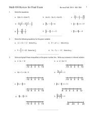
“Graphical Solutions to Equations”30plot of x 3 and 20*cos(x)20100about 1.4−10about −2.0−20about −2.5−30−3 −2 −1 0 1 2 3Figure 1: Plot of x 3 and 20 cos(x). The solutions to the equation x 3 = 20 cos(x) are the xvalues of the intersection points.Step 1. Plan you actions We will graph both f(x) = x 3 and g(x) = 20 cos x and look for intersectionpoints. Alternatively, you could plot f(x) = x 3 −20 cos(x) and look for its zeroes.To find an appropriate viewing window, we notice that when x = 3 we have x 3 = 27 whichis already more than 20, the largest 20 cos(x) can be. By symmetry, we will choose theinterval [−3, 3] for our initial plot (Figure 1). If this isn’t large enough, or is too small wewill make an adjustment and replot.Step 2. Make the plot(s) The graph is created with these commands>> x = linspace(-3,3);>> y1 = x.^3;>> y2 = 20*cos(x);>> plot(x,y1, x,y2)You could also use hold here and make the plots incrementally.Step 3. Investigate the graph Looking at the graph, we can see that the solutions are about−2.5, −2.0, and 1.4, but we can do better by zooming in around these intersection points.Step 4. Zoom in Let’s find the value of the root near 1.4. First we check if 1.4 is very close bylooking at the difference between the two functions:http://www.math.csi.cuny.edu/matlab project 4 page 2

“Graphical Solutions to Equations”>> x = 1.4x = 1.4000>> x^3 - 20*cos(x)ans = -0.65534We are not very close. We turn the zoom feature on using the magnifying glass icon, or thezoom function and then click near the intersection point. The plot is redrawn with half the xand y axes. We see the answer is closer to 1.42. Clicking again, we see that a value of 1.425seems about right. We check to see how close we are>> x = 1.425x = 1.4250>> x^3 - 20*cos(x)ans = -0.0120It is not exact (1.4255 is closer), but we have to be careful when we zoom in too close,as our graph may not accurately portray the actual function. Recall we have plotted 100points evenly spaced between -3 and 3 so that roughly there are 16 points between 1 and2. After zooming in this closely, the plot is made up of just a few line segments, whereasthe functions’ graph is actually a curve. To get more accuracy, it is best to replot with morepoints in the neighborhood of the answer you are looking at.Although zooming is valuable to quickly find pretty good answers, there are other methodsfrom numerical analysis which are more accurate. In a later project we explore one calledNewton’s method.Exercise 1:Use a graph of (x − 2) 2 = 4 sin(x) to find solutions to the equation valid to 2 decimal points:(1) Answer:Exercise 2:Use the zooming technique to find solutions of50 + sin x = 2x.which are valid to at least two decimal places.Hint: Try to estimate the value of 50 + sin x. This will give you an idea in which x interval are thepossible solutions!(2) Answer:http://www.math.csi.cuny.edu/matlab project 4 page 3

“Graphical Solutions to Equations”Exercise 3:Folklore is that exponential functions grow faster than polynomial functions. Although true, youneed to be careful about how you interpret this statement, as this exercise shows.Consider the functions z 1 = e x and z 2 = x 4 . Plot them together on the interval [0,4].a. From their graphs, how can you determine which graph is the exponential and which is thepolynomial?(3) Circle one:1. polynomial functions grow faster than exponential functions2. Exponential functions grow faster than polynomial functions3. For different values of x, I can evaluate z 1 , z 2 and determine which is larger.b. Find the value of x (to two decimal places) for the point of intersection by zooming on thezero of f(x) = e x − x 4 . (or by zooming on the intersection point of the functions z 1 = e x ,z 2 = x 4 .)(4) Answer:On this graph, x 4 is larger than e x from the intersection point to x = 4. Experiment todetermine how large a value of x is needed for the exponential to catch up to x 4 . Then findthe second intersection point. (correct to three decimal places.) This one is larger than 4. Infact, you now have found two intersection points (x 1 , y 1 ), (x 2 , y 2 ). (where x 1 < x 2 ) Up to x 1the function e x is bigger, from x 1 to x 2 the function x 4 is the bigger. What happens after x 2 ?c. What is the x-coordinate of the second intersection point?(5) Answer:d. What happens to the behavior of z 1 and z 2 after the second intersection point?(6) Circle one:1. e x grows faster2. x 4 grows faster3. they grow at the same rate4. e x grows faster, but for increasingly large values of x, x 4 catches up to e x again.Vertical asymptotes can be a real impediment to finding roots, as this example illustrates.Example 2:Find any zeroes and the minimum value of the rational functionf(x) = x + 2x 2 .We first graph the function over initial interval [−10, 10] producing Figure 2.http://www.math.csi.cuny.edu/matlab project 4 page 4

“Graphical Solutions to Equations”250200150100500−50−10 −8 −6 −4 −2 0 2 4 6 8 10Figure 2: The function f(x) = (x + 2)/x 2 illustrating a vertical asymptote.The figure illustrates that the vertical asymptote at x = 0 gets in the way of finding the twoanswers we want—the zeroes and the minimum value. Let’s try again using a little thought beforewe chug ahead with the computer.Recall that rational functions are 0 only when the numerator is, that is when x + 2 = 0, orx = −2. The function goes from negative to positive there, so the minimum must be located to theleft of −2. As this function has a horizontal asymptote of y = 0 there must be a minimum to theleft of −2, and no minimum to the right of 0 where the function is positive. You’ll do the rest inthe following exercise.Exercise 4:a. Find the x-coordinate for where f(x) = (x + 2)/x 2 achieves its minimum value.(7) Answer:b. What interval on the x-axis did you use to make you plot window?(8) Answer:http://www.math.csi.cuny.edu/matlab project 4 page 5

“Graphical Solutions to Equations”3 Finding roots of polynomialsPolynomial functions are extensions of linear and quadratic functions (a ≠ 0):f(x) = ax + b, (linear) f(x) = ax 2 + bx + c (quadratic).For these two types of functions we can solve f(x) = 0 easily. For the linear case the singlesolution is −b/a. For the quadratic case the quadratic formula produces two answers. Theseanswers are the roots of the polynomial.The quadratic formula produces two roots, although many possible cases exist: two distinctreal roots, double roots, or two complex-valued roots that come in conjugate pairs. There are alwaysno more than 2 real roots.A general polynomial of degree n may be written asf(x) = a n x n + a n−1 x n−1 + · · · a 2 x 2 + a 1 x 1 + a 0 .For an nth degree polynomial there are n, possibly complex, roots counting multiplicities. Butthey need not all be real roots. However, there is not always a formula for solving for these roots.However, MATLAB has a built-in function, called roots, that numerically solves for the roots,which is faster and more accurate than the zooming technique. To use roots, you must code thepolynomial f(x) like a vector. We take each coefficient (there are n + 1) and enter them in orderas follows:The polynomial f(x) is represented with>> p = [a n a n−1 · · · a 2 a 1 a 0 ]Then the polynomial equation f(x) = 0 is solved with the command>> roots(p)The only subtlety is that we don’t usually write the terms whose coefficients are 0, but we mustdo so when entering in the polynomial into MATLAB. So, for instance[3 2 1] represents f(x) = 3x 2 + 2x + 1,[3 2 1 0] represents f(x) = 3x 3 + 2x 2 + x,[3 2 0 1] represents f(x) = 3x 3 + 2x 2 + 1, and[3 0 0 2 1] represents f(x) = 3x 4 + 2x + 1.Example 3:Use the roots function to find the roots of f(x) = 2x 3 + 6x 2 − 4x − 5.>> p = [2 6 -4 -5]p =2 6 -4 -5>> roots(p)http://www.math.csi.cuny.edu/matlab project 4 page 6

“Graphical Solutions to Equations”ans =-3.37321.0675-0.6943We get 3 real roots. We could verify this by plotting the polynomial over the interval [−4, 2]and observing the graph crosses the x axis three times. Instead, we illustrate that these are roots,by evaluating the polynomial at these values:>> x = roots(p) % store the values>> 2*x.^3 + 6*x.^2 -4*x -5 % evaluate the polynomial for rootsans =1.0e-13 *-0.31970.04440These values are very close to 0, as they are multiplied by 1.0e-13. This is MATLAB’s scientificnotation for 10 −13 .Exercise 5:a. Let f(x) = x 3 − 7x 2 + 2x + 9. Solve the cubic equation f(x) = 0. Find all of its rootscorrectly up to 4 significant digits.(9) Circle one:1. 6.6 , 1.1 -0.72. 6.4766, 1.4692, -0.94583. 6.7053 , 1.3259 , -0.82594. 0.0010, 1.0100, 7.59025. 6.5806 , 1.1062, -0.6868b. Now find all solutions to x 3 + 2x + 4 = 0 (Note that the coefficient of x 2 is now 0).(10) Circle one:1. 0.6641, -0.6640, -1.32832. 1.8230, -1.8230, -1.32833. 0.5898 ± 1.7445i −1.17954. 1.8230 ± 0.6641i , -1.3283This last exercise illustrates that both means of finding zeroes of functions can be useful.http://www.math.csi.cuny.edu/matlab project 4 page 7

●●●●●●●●●●●●●●●●●●●●●●●●●●●●●●●●●●●“Graphical Solutions to Equations”Example 4:The flight of an arrow through space can be modeled with or without air resistance. How do themodels differ?An arrow's flightyθxFigure 3: Flight of an arrow without air resistance.When an arrow encounters no air resistance the laws of projectile motion from high-schoolphysics apply. Using x for the horizontal distance traveled, f(x) for the height of the arrow whenit is x units away, and θ for the initial angle, we have this model for the trajectory of an arrowwithout air resistance:(f(x) = tan θx − 16x200 cos θ) 2When there is a drag on the arrow proportional to its velocity (k is the proportion factor), theheight of the arrow is given by:32g(x) = tan(θ)x +k200 cos θ x − 32 ()200 cos θk log .200 cos θ − xFor both models, the range of flight is the time that y ≥ 0. (When y ≤ 0, the definition of bothg(x) and f(x) should be set to 0.) The range can be written as [0, b].First, we investigate an arrow’s flight without wind resistance.http://www.math.csi.cuny.edu/matlab project 4 page 8

“Graphical Solutions to Equations”Exercise 6:a. Let θ = π/4. Look carefully at f(x), it is a quadratic polynomial in x. Rewrite f(x) so thatthe coefficients appear as (careful with the scientific notation)f(x) = ax 2 + bx + c.Now represent this polynomial in MATLAB, as in [a b c]. What are the values:(11) Answer:b. Use your previous answer and the roots function to find the range ([0, b]) of an arrow whenshot at an angle of π/4. Specify the range in terms of its endpoint b.(12) Answer:Next, we consider the model with wind resistance. To keep matters simple, we assume k = 1/2.Then our formula for the trajectory when θ = π/4 becomes, in MATLAB,>> theta = pi/4;>> k = 1/2>> a = 200*cos(theta);>> b = 32/k;>> g = (tan(theta)+ b/a)*x - b*log(a ./(a-x));provided you have defined values for x.http://www.math.csi.cuny.edu/matlab project 4 page 9

“Graphical Solutions to Equations”Exercise 7:a. Plot various graphs of the g(x) until you find the range of g, [0, b]. Enter the value of b withat least 1 digit to the right of the decimal point. (Remember, arrows don’t bounce up – thismathematical model is only valid until the arrow first hits the ground.)(13) Answer:b. Now make a plot containing the trajectories of both models. Label the individual plots.(14) Attach your graph to the worksheet.c. From your graph estimate the maximum height of the arrow if there is no wind resistance.(15) Answer:d. From your graph estimate the maximum height of the arrow if there is wind resistance.(16) Answer:4 Extra credit problem(To be handed in on a separate sheet of paper.)It can be shown that the maximum range for the arrow if there is no wind resistance happenswhen θ = π/4. However, this is not the case for the model with wind resistance. By exploringaround with different values of θ, find a value of θ that maximizes the trajectory.http://www.math.csi.cuny.edu/matlab project 4 page 10

“Investigating Limits in MATLAB”MTH2291 IntroductionThe College of Staten IslandDepartment of MathematicsInvestigating Limits in MATLABIn this lesson, we learn how to investigate limits of functions using MATLAB. First a review ofsome key facts about limits.For continuous functions it is easy to find a limit becauselim f(x) = f(c).x→cThis is sometimes called “plugging in,” as the limit at c is simply the value of the function at c.Graphically, we find the limit at c by observing the corresponding y value at cOther functions are not continuous at a point c, but would be if the function could be redefinedat c. These values of c may be called removable singularities. Although the function is not definedat c, we can still find the limit graphically. Simply follow the graph over to where the functionshould be defined at c to make it continuous.Some functions have only right or left limits at a point c. This means we don’t look on bothsides of c to investigate the functions behavior, rather only one side. Of course, a function has alimit only if it has a left and right limit and the two are the same. Left and right limits may beinvestigated graphically, by plotting the graph of the function on just one side of c.We can also investigate limits using a table. The limit of f(x) at c is intuitively the value thatf(x) approaches as x approaches c. Often we can take x close to c and then f(x) will be close tothe limit lim f(x) as x → c. We can make a table of values getting close to c and a correspondingtable of function values, and look for trends.This project will investigate limits both graphically and numerically. As well, as a useful aside,we will learn how to define functions in MATLAB so that our work can be simplified.1.1 New MATLAB topicsa. Function m-files (script files too)b. format [long short] – control the format of MATLAB’s answers2 Finding limits with MATLABWith MATLAB we can’t use the ɛ–δ definition of a limit, but rather rely on what the limit of afunction tells us, namely as x approaches c the function approaches the limiting value.http://www.math.csi.cuny.edu/matlab project 5 page 1

“Investigating Limits in MATLAB”As an example, we illustrate how to find the following fundamental limit using MATLAB:sin xlimx→0 xFirst we note that this function, f(x) = sin(x)/x is continuous everywhere except at c = 0, sotrying to “plug in” will fail. To see how, we try use MATLAB:>> x=0; sin(x)./xWarning: Divide by zero.ans = NaNHmmm, Not a Number. As expected.A plot of the function near 0 may be illuminating. Although we only need to plot the functionnear 0, we show in Figure 1 the interval from −2π to 2π so that we can see that this functionoscillates like a damped sine curve, except near 0 where the limit can be seen to be 1.>> x = linspace(-2*pi,2*pi) % numbers around 0.>> plot(x,sin(x)./x)How come there is no error message when x = 0? This is because 0 is not one of the valuesin x. We need to take an odd number of points to make that happen, as you can verify if you wereto use linspace(-2*pi,2*pi,101) for x. What happens instead of an error is that the pointsnearby 0 get connected with a line. As this point of discontinuity is a removable singularity, thegraph appears to be continuous, as though f(x) were defined to be 1 at 0.1Graph of sin(x)/x. The limit at 0 is 1.0.8Function is undefinedat x=0. But is continuousif you let it be 1 at x=0.Limit as x−> 0 is 10.60.40.20−0.2−0.4−15 −10 −5 0 5 10 15Figure 1: Plot of f(x) = sin x/x showing a limit of 1 at c = 0.http://www.math.csi.cuny.edu/matlab project 5 page 2

“Investigating Limits in MATLAB”2.1 Finding limits using tablesHow might we have found this value numerically? The basic idea is that to investigatelim f(x)x→cwe look at values of x “close” to c and compare what the corresponding f(x) values get “close”to.To take x values close to c can be done by hand as with>> x = [.1 .01 .001 .0001 .00001];The corresponding values of f(x) are then>> y = sin(x) ./x;To see them in a table format for easy comparisons we use the following notation:>> format long %14 digits to right of decimal point>> [x; y]’ % a semicolon and a ’ans =0.10000000000000 0.998334166468280.01000000000000 0.999983333416670.00100000000000 0.999999833333340.00010000000000 0.999999998333330.00001000000000 0.99999999998333 % y values get close to 1The tables shows that f(x) gets close to 1 as x gets close to 0 from the right. We should checkthe values from the left side of 0 as well, but in this case we merely note that f(x) is an evenfunction so a left limit at 0 will exist and be the same as the right limit.You can toggle between showing 4 or more decimal places using the commands>> format short % show fewer decimal places>> format long % show more decimal placesOne caveat, when looking for convergence, you may not find it if there are numerical instabilities.Exercise 1:Use the graphical approach to find the following right limit of f(x) = x x , x > 0limx→0 + xxWhat is the value of the limit?(1) Answer:http://www.math.csi.cuny.edu/matlab project 5 page 3

“Investigating Limits in MATLAB”Exercise 2:a. Use the numeric approach to find the following limit1 − cos(x)limx→0 x 2What is the value of the limit?(2) Answer:b. Numerically investigating a limit at a point c which is not zero requires us to use pointswhich get close to c. A simple trick allows us to reuse our points which get close to 0. Forinstance if>> x = [.1 .01 .001 .0001 .00001]; % and>> c = 1/2;Then we can make points getting close to c from above and below as follows:>> c + x; % points above c>> c - x; % points below cUse this to investigatelim ( π − x) tan(x).x→ π 22What value for the limit do you get? (Enter no limit as DNE.)(3) Answer:Exercise 3:To illustrate what can happen numerically with some functions, we again look at finding the limit1 − cos(x)lim .x→0 x 2Only we let x get really close to 0. First we use some MATLAB shortcuts to define increasinglysmaller values in x>> n = 1:8; x = 10^(-n); % Small valueshttp://www.math.csi.cuny.edu/matlab project 5 page 4

“Investigating Limits in MATLAB”0.5Graphical approach and the points fromthe numeric approach.0.4950.490.4850.48points used in table givea bad graph.0.4750.470.4650.460.455−1 −0.8 −0.6 −0.4 −0.2 0 0.2 0.4 0.6 0.8 1Figure 2: Figure illustrating graphical and numeric approach to solving a limit. Notice thex values chosen for the numeric are bad values for making the graph of the function.Now produce a table of the f(x) values for these values of x. Use this to investigate the limitat 0 of the function. How does the numerical instability of the problem show up in the output?(4)Exercise 4:Let f(x) = x ln(x),x > 0. Calculate the following right limit with MATLAB as directed:lim f(x).x→0+a. Use a vector of numbers that converge to 0 from the right to investigate numerically the limitas x goes to 0. What is your numeric estimate for the limit?(5) Answer:b. Enter in your table of values here. (Use the syntax [x;y]’.)(6)http://www.math.csi.cuny.edu/matlab project 5 page 5

“Investigating Limits in MATLAB”c. Plot a graph of f(x) over (0, 1). Does the graph confirm your limit found from the table ofnumbers?(7) Circle one:1. Yes 2. Nod. Although the function is only defined for x > 0, plot a graph of f(x) over (−1, 1). Does thegraph show anything unusual?(8)Example 1:Unfortunately, not all graphs will immediately give us an answer. This example illustrates a possibletrouble identifying a limit from the graph and then shows how a theorem from calculus canhelp us figure out the actual limit.We wish to find the limit of the oscillating function( 1f(x) = x sinx)as x approaches 0.Exercise 5:Plot the function f(x) = x sin (1/x), over the interval [−π, π] using 100 points for x.a. Try to zoom in on the limit. What happens near x = 0 that prevents you from getting thecorrect answer?(9)b. Graph the same function using 1000 points on top of your current graph (hold) using adifferent color.http://www.math.csi.cuny.edu/matlab project 5 page 6

“Investigating Limits in MATLAB”c. The graph with 100 points didn’t allow us to zoom in far enough to see the limit as thisfunction oscillates so often that when we zoom in we eventually get just straight lines.Do you have this same problem using 1000 points?(10) Circle one:1. Yes2. Nod. Motivated by the squeeze theorem, on the same graph (hold on) plot both y = |x| andy = −|x| (|x| is abs(x) in MATLAB) What relationship, if any, can be observed betweenf(x) = x sin (1/x) and these two lines?(11) Circle all that apply:1. |x| ≤ f(x)2. |x| ≥ f(x)3. −|x| ≤ f(x)4. −|x| ≥ f(x)e. Graphically estimate the limit as x → 0 What is the limit?(12) Answer:f. How did graphing the absolute value functions help you find the limit?(13) Circle one:1. The mean-value theorem2. The function is continuous3. the squeeze (or sandwich) theorem4. they didn’t I just guessed3 Using FunctionsA mathematical definition of a function f(x) is that it is a rule that assigns to each x in its domaina single value y in its range. We might call x the input and y the output. We use functions for manyreasons. First they allow us to generically talk about problems. So instead of saying lim x 2 −2x wecan talk about lim f(x). This makes it easier to make general statements and to identify the typeof problem we may be encountering. As well, functions allow us to simplify our work. Instead ofwriting out the function definition each time, we can simply refer to it by its name.Using MATLAB we seek the same abilities. MATLAB provides a mechanism to define functions,we which explain quickly below. More details are provided at the end of the project.http://www.math.csi.cuny.edu/matlab project 5 page 7

“Investigating Limits in MATLAB”First we break the function into its three pieces: its input, its rule, and its output. Our basictemplate for defining a function will look likefunction outputVariable = functionName( inputVariable(s) )outputVariable = rule depending on inputVariable(s)Usually the output variable and input variables are simply named, like x or y. For instance, thiswill define a MATLAB function to evaluate f(x) = sin(x)/x:function y = f(x)y = sin(x) ./ x;This function template will define the function g(x) = 7x 2 sin(1/(7x 2 )):function y = g(x)a = 7*x.^2;y = a .* sin(1./a);A few things to note, the first line has g(x) as we want to call this function by the name g.Second, the rule here uses two lines, as the function naturally lends itself to two pieces. This is notan issue, the last definition for y, the output variable, is what gets returned.The main features of our function template are:The keyword function The first (non-comment) word is the keyword function which tellsMATLAB that we are defining a function.The name of the function The name that we will use to call this function appears in the firstline. In the two examples, the names are f and g.The definition of the input and output variables The output variable is defined just afterthe function keyword. We will always use y for the name, but this is only by convention,more complicated return values are possible. The value returned by the function is the lastdefinition of this variable within the body (the rule) of the function.The input variable(s) are specified after the name of the function and within parentheses. Inour examples there is only 1 input variable, more are possible.The body of the function The function’s rule is defined in the body of the function. You canuse the input variable names inside the body. You must take care to assign a value to theoutput variable in the body of your function if you want to return any information. We putsemicolons after each line in the body to keep things quiet, otherwise MATLAB will printthe value of each line while processing the function.Now where do we define a function? It would be convenient to do so at the command line, butwe can’t. Instead MATLAB has a different mechanism involving files on the harddrive. These arecalled m-files, as their extension will always be .m. The basic idea is as follows: (cf. Figure 3)http://www.math.csi.cuny.edu/matlab project 5 page 8

“Investigating Limits in MATLAB”a. We open a file and type in our function template. Suppose the name is f. MATLAB hasa built in editor for editing functions (like notepad, only better). This editor uses tabs sothat many functions may be edited at once. It is found under the File menu of the mainMATLAB window.To open a new m-file you use the New->M-file menuitem. To open an existing m-file youuse the Open... dialog.b. We save the file as f.m; we have no choice if we used the name f when defining the function.The file should be saved in the default directory provided by the MATLAB function editor.This way MATLAB can find the function when it is requested.You do not need to close the m-file editor after working on the file.c. We use the function by its name as we would any other function. That is, using parenthesesand with arguments.Define a functionusing MATLAB’seditorUsing at command line−−−−−−−−−−−−−−−function y = f(x)y=sin(x)./x;Store on hardriveasf.m−−−−−−−−−−−−−−−>> x = linspace(−pi,pi);>> plot(x,f(x))Figure 3: The three aspects to defining a function: the function template (with name), thenaming of the m-file storing the function, using the function with a MATLAB sessionSuppose we followed the instructions above and saved our template that defines f(x) =sin(x)/x in a file f.m. Then we can use our function as follows:>> f(1) % call with a fixed valueans = 0.8415>> x=1;f(x) % call with an assigned variableans = 0.8415>> x=[1,2,3];f(x) % call with a vectorans = 0.8415 0.4546 0.0470>> f % needs a value as input to f.m??? Input argument ’x’ is undefined.http://www.math.csi.cuny.edu/matlab project 5 page 9

“Investigating Limits in MATLAB”Exercise 8:a. Find the following limit using composition of functions:lim g(f(x))x→0+What is the value of the limit?(17) Answer:b. There are many consequences of the definition of limits that make finding limits easier. Forinstance, the limit of a sum is the sum of the limits (provided all the limits exist). Another isthe limit of compositions can be expressed in terms of the limits. That is, iflim f(x) = L,x→cand lim g(x) = M,x→Lthenlim g(f(x)) = M.x→cVerify that this is the case with f and g defined as in the last problem. Is it true?(18) Circle one:1. yes 2. noExercise 9:The derivative of a function g(x) at x is given by the following limitThe derivative at x = limh→0g(x + h) − g(x)hLet g(x) = x x . This should be defined in a function m-file called g. If not, do so now.a. Find the derivative of g(x) at x = 1 by investigating the above limit. Use the expression>> y = (g(1+h) -g(1)) ./hrather than doing the composition and secant line expression directly from the function definition.What is the value of the limit?(19) Answer:http://www.math.csi.cuny.edu/matlab project 5 page 11

“Investigating Limits in MATLAB”b. Now we try to to find the right limit of the derivative formula when x = 0. As g(0) is notdefined, we replace it with it’s limit of 1.What do you find when investigating(20)limh→0+g(h) − 1?h4 Function specificsMATLAB’s mechanism for functions is an “m-file”. More generally, an m-file is one of MAT-LAB’s ways of storing information to a disc drive (others are save and load). They are calledm-files because they are saved with the extension .m (for example function.m). They come intwo flavors,• script m-files: these save a fixed sequence of commands.• function m-files: these save functions. A function takes some input (which is in a domain)and after evaluating some commands, returns the output (in its range).Both are similar: they are both text files stored with the special suffix .m. We will just discussfunction m-files.Script m-files Script m-files are simply a way to store commands in a file that will get executedall at once. They are a convenient way to do work if it involves many lines of evaluation aserrors can be easily fixed.To use a script m-file you need toa. Create a file (say script.m) with the commands you want to execute.b. Save this in the correct place, or tell MATLAB where it is by using the cd command tochange to the directory the file is in. The following will cd to the “a” drive and look forfiles there.cd a:Alternatively, you can tell MATLAB where your file is by setting the path. This isdone with a command like the following which adds the “a” drive to the path.>> path(path,’a:\’)http://www.math.csi.cuny.edu/matlab project 5 page 12

“Investigating Limits in MATLAB”c. Execute the commands stored in the script file by calling the name from the commandline without the .m extension. For example, if the file is called script.m, then thecommand line>> scriptwill run the commands.Function m-files Function m-files are very similar to the above, except they let you pass invalues and return values. The simplest instance would be to mimic a mathematical functionsuch as f(x) = sin 2 (x).To make a function m-file for this we would create a file f.m with these contentsfunction y = f(x)y = sin(x).^2;We save the file. If we put it in the correct place, then running this file is easy, just like aregular MATLAB function. That is, we use parentheses and numbers. For example>> f(2)5 Functions can save work. Really!Here is a sample function which can actually save time! To graph a function in MATLAB issomewhat tedious. You need to define x usually with linspace, then define y, and then define theplot commands. Here is a function which will do this all for you. Save this function as plotf.mfunction y = plotf(a,b,n)% plotf: plots f over [a,b]. f is an m-file previously definedif (nargin

“Investigating Limits in MATLAB”function y = f(x)% this is a functiony=x.^2;then from the command window we would have>> help fthis is a functionError messages when calling the file It is important to remember that script m-files andfunction m-files are called in different manners. If you have an m-file called f.m then if it isa script m-file it is called on the command line with>> fWhereas, if it is a function m-file, doing this will cause an error. Functions need to havearguments. You call them like>> f(x)where x is some previously defined number or list of numbers.MATLAB can’t find your m-file MATLAB has a path that it uses to search for files. Ifyour file isn’t on the path, MATLAB won’t know about it. To ensure that your file is onthe path you can change to the current directory. For example, if the file is on a diskette,then the command cd a:\ should suffice. Otherwise you can adjust the path variable with>> path(path,’a:\’).MATLAB can find a file, but it doesn’t look like mine When MATLAB looks alongits path for a function or script file, it finds the first thing it can. In particular, if someonehas an m-file with the exact same name as yours, but it appears first on the path, then thatm-file will be the one executed. Usually, the current directory is first on the path, and so thecd command above will usually suffice.MATLAB can’t find your script file The syntax to call a script file is identical to that toview the contents of a variable. This is not a problem unless you have a variable with thesame definition as your script m-file. In this case the variable’s contents are given and notyour script file.MATLAB finds a variable before a function If you happen to have a variable with thesame name as your function, then the variable will be returned. For example, suppose youhave an m-file f.m containingfunction y = f(x)% this finds x e^(1/x)y = x.* exp(1 ./ x);http://www.math.csi.cuny.edu/matlab project 5 page 14

“Investigating Limits in MATLAB”Then we would have the following session>> f(2) % call the functionans = 3.2974>> f = 1 % set a variable ff = 1>> f % view the variablef = 1>> f(2) % it tries the variable not the function??? Index exceeds matrix dimensions.>> clear(‘‘f’’) % clear the variable. Oops??? clear(‘‘f |Use single quote character instead of double quote or backward quote.>> clear(’f’) % Okay, single quotes.>> f(2) % Now it works againans = 3.2974http://www.math.csi.cuny.edu/matlab project 5 page 15

“Approximate First and Second Derivatives”MTH2291 IntroductionThe College of Staten IslandDepartment of MathematicsApproximate First and Second DerivativesThe derivative of a function f at x is defined in terms of a limit, which may be written asf ′ f(x + h) − f(x)(x) = lim.h→0 h4f(x) = x x and the tangent and some secant lines at x 1= 0.6.3.532.521.5h=1 h=.51tangent line0.5(.6,f(.6))0−0.50 0.2 0.4 0.6 0.8 1 1.2 1.4 1.6 1.8 2Figure 1: Graph of the function f(x) = x x over [0, 2]. Layered on top are the tangent lineat x = 0.6 and two secant lines corresponding to h = 1.0 and h = 0.5. As h approaches 0,the slope of the secant line approaches the slope of the tangent line.The expression that we take the limit of,f(x + h) − f(x)his interpreted as the slope of the secant line that goes through the points (x, f(x)) and (x+h, f(x+h)). Then the derivative is interpreted as a slope, in this case of the tangent line, defined as thelimit of the slopes of the secant lines.http://www.math.csi.cuny.edu/matlab project 6 page 1

“Approximate First and Second Derivatives”We’ve seen that MATLAB can be used to investigate limits. Although, MATLAB doesn’tactually find the limit, it suggests an answer by being close to the true answer. In this same way,MATLAB can help us find the value of the derivative of f(x) at a single point, and as a function ofx (many points at once.)Figure 1 shows that graph of f(x) = x x over the interval [0, 2] along with three lines which gothrough the point (0.6, f(0..6)). The tangent line is drawn to have slope given by f ′ (x) evaluatedat 0.6. The secant lines are drawn to have slope which depends on a specified value of h. Forinstance, when h = 1 the slope isf(0.6 + 1) − f(0.6)1=2.1213 − 0.73601= 1.3852.Clearly this is not close to the derivative, since the slope of this secant line is not close to the slopeof the tangent line. We don’t expect it to be, as h is not close to 0. Taking values of h getting closerto 0 allows us to approximate the derivative at 0.6:>> c = 0.6; h = [1.0 0.1 0.01 0.001 0.0001];>> y = ( (c+h).^(c+h) - c^c ) ./h;>> [h; y]’ans =1.0000 1.38520.1000 0.43030.0100 0.36710.0010 0.36070.0001 0.3601We’ll take the value f ′ (0.6) = 0.3601 as the approximate derivative. This is about as good as wecan get before learning how to find the actual derivative algebraically.The same approach to finding limits can be done for many x values at once. This allows us tograph an approximation to the actual derivative of a function f. As well, we’ll see how to plot anapproximate second derivative. We emphasize that these are approximate, as we will use a fixedvalue of h, which although small, is still not “going to” 0.2 The derivative at a pointExercise 1:Let f(x) = sin(x 2 ). We wish to find the derivative of f when x = π/4.a. Make a function m-file storing the function f(x) = sin(x 2 ) with name f.m. What are thecontents of the file:(1)http://www.math.csi.cuny.edu/matlab project 6 page 2

“Approximate First and Second Derivatives”b. Take h = 0.1 and find the slope of the secant line at (x, f(x)):(2) Answer:f( π + h) − 4 f(π)4.hc. Take smaller values of h to find a better approximation to f ′ (π/4) (Four decimal points ofaccuracy is good.)(3) Answer:Exercise 2:We will see how the secant line approaches the tangent line for the function f(x) = sin(x) at thepoint x 1 = π/4. Do this by following this sequence of steps. When you are done you will uploadyour graph to show your work.A secant line is just a line drawn between two points on the graph of f(x), where one of thepoints is the point of interest like x 1 = π/4 in this example. The second point can be called x 2 ,but we prefer to emphasize its relationship to x by writing x 2 = x + h where h then is the distancebetween the two points.a. Make a function m-file storing the function f(x) = sin(x) with name f.m. What are thecontents of the file:(4)b. Graph f(x) over the interval [0, π].c. Let h = π/2. On your graph, add the secant line connecting the points x 1 = π/4 andx 2 = x 1 + h = 3π/4.The following commands will help you plot such a line.>> x1=pi/4;>> h = pi/2; x2 = x1+h; m = (f(x1+h)-f(x1)) / h ;>> plot(x, f(x1) + m*(x-x1)) % point-slope form of line>> plot(x2,f(x2),’*’) % mark the pointWhat is the slope of this secant line?(5) Answer:d. For h = 0.1, and h = 0.001 draw the secant line as above. Label the different secant lineswith the value of h.http://www.math.csi.cuny.edu/matlab project 6 page 3

“Approximate First and Second Derivatives”e. The tangent line at x 1 = π/4 has slope √ 2/2. Plot the tangent line on the same graph in adifferent color and label it.f. Submit the graph of Example 1.(6) Attach your graph to the worksheet.g. Explain carefully the relationship between h and slope of the secant lines for h. In particular,what is the limit of these slopes as h gets closer to 0?(7)3 Derivative of a FunctionWe’ve seen that the derivative of f(x) at c is approximately given by (f(c + h) − f(c))/h for smallvalues of h. To find the derivative of a function for many x values at once, we simply fix a singlesmall value of h, and use many values for c. We call this approximate derivative the differencequotient:difference quotient =f(x + h) − f(x)hsmall h.Example 1:(Graphing the difference quotient)Let us create a plot of the derivative of f(x) = cos x over the interval [0, 2π] based on the numericalevaluation of its difference quotient. We shall use h = 0.01 in evaluating the difference quotient.The following MATLAB commands will plot both the function and its approximate derivativetogether over the interval [0, 2π].>> h=0.01; % a small value for h>> x=linspace(0,2*pi); % lots of x values>> difquo=(cos(x+h)-cos(x))./h; % difference quotient. Or use an m-file>> plot(x,cos(x),’r’,x,difquo,’b’),grid % plot cos in red and difquo in blueExercise 3:Have a close look at the resulting graphs of Example 2. Identify which is the graph for cos(x)and which is the graph for difquo.http://www.math.csi.cuny.edu/matlab project 6 page 4

“Approximate First and Second Derivatives”a. Does the graph of difquo resemble the graph of a function that you are familiar with?(8) Circle one:1. sin x2. − sin x3. cos x4. − cos xb. Based on your answer to part 1, what do you think is the derivative of y = cos x?(9) Circle one:1. sin x2. cos x3. − cos x4. − sin xExercise 4:It is known that the derivative of the function f(x) = x 3/2 + 5 is given by f ′ (x) = 3/2 √ x. Wewill verify that the difference quotient converges to this function as h goes to 0 over the interval[0, 2]a. Write an m-file storing the definition of f(x). List its contents here:(10)b. For h = 0.1 make a graph of the difference quotient and the derivative. What is the largestdifference between the two functions?(11) Answer:c. On the same graph, plot the difference quotient for h = 0.001. What is the maximumdifference now between the difference quotient and the derivative function?(12) Answer:Exercise 5:Numerical differentiation of exponential functionYou may not know the derivative of f(x) = e x and g(x) = ln(x) at this point. Let’s use thedifference quotient to figure out the derivative of e x .http://www.math.csi.cuny.edu/matlab project 6 page 5

“Approximate First and Second Derivatives”a. Use MATLAB to create a continuous plot of f(x) = e x over the interval −2 ≤ x ≤ 2. Basedon this graph, which of the following should be true about the derivative.(13) Circle all that apply:1. f(x) is always increasing so f ′ (x) > 0.2. Tangent lines for f(x) are never ’flat’ so there are no critical points.3. f(x) increases faster and so f ′ (x) should be increasingb. On top of the graph of f(x), create a plot of the difference quotient of f(x) using h = 0.01over the same interval [−2, 2] in a different color. Turn in your graph.(14) Attach your graph to the worksheet.c. Based on the two plots, what do you think the derivative of f(x) = e x is.(15) Circle one:1. x e2. log x3. x 2 4. e x4 The approximate second derivativeThe second derivative is approximated in a similar way as the first derivative is approximated. Acommon approximation is given bydifdifquo =f(x + h) − 2f(x) + f(x − h)h 2 .It can be checked that as h approaches 0, the difdifquo (for lack of a better name) convergesto f ′′ (x).Using an m-file makes it easier to find the approximate second derivative. For instance, thefollowing example will plot a function f(x) and its approximate second derivative over the interval[0, 1]. It just needs an m-file defining the function f.>> x = linspace(0,1); % adjust for your problem>> h = 0.01; % a small enough number?>> plot(x,f(x),x,(f(x+h) - 2*f(x) + f(x-h))/h^2,’g’),gridThat’s it.http://www.math.csi.cuny.edu/matlab project 6 page 6

“Approximate First and Second Derivatives”Exercise 6:We wish to graph the function f(x) = e x/3 sin(πx).a. Write an m-file that evaluates this function. Call your m-file f.m.(16)b. Make a plot of f(x) over the interval [0, 3].c. Using h = 0.01 compute the difference quotient for x in the interval [0, 3]. Write down thecommands to find the difference quotient and add its graph to the graph of f(x).(17)d. Again using h = 0.01, find the approximate second derivative (difdifquo) and add its plotto your plot of the function. What are the commands you used to find difdifquo?(18)e. Use an arrow to label any zeroes of the approximate first derivative on your graph. What canyou say about the graph of f(x) near these x values?(19)f. Submit your three graphs in one figure with the requested annotations.(20) Attach your graph to the worksheet.http://www.math.csi.cuny.edu/matlab project 6 page 7

“Critical and Inflection Points”MTH2291 IntroductionThe College of Staten IslandDepartment of MathematicsCritical and Inflection PointsThis project explores the important relationships between a function, f(x), and its first and secondderivatives, f ′ (x) and f ′′ (x). For instance, we know:• f ′ (x) is positive on an open interval is equivalent to f(x) is increasing on the interval.• f ′ (x) is increasing on an open interval is equivalent to f(x) being concave up on the interval.• f ′′ (x) is positive on an open interval is equivalent to f(x) being concave up on the interval.These facts lead to the first and second derivative tests, which allow us to check if a criticalpoint is indeed a relative maximum or a relative minimum. Recall, a critical point, c, is a value inthe domain of f(x) where f ′ (c) = 0 or f ′ (x) is undefined at x = c.2 The first derivativeWe investigate the functionf(x) = 4x 4 − 12x 3 + 9x 2 .>> x=linspace(-3,3);>> y=4*x.^4 - 12*x.^3 + 9*x.^2;>> plot(x,y), gridA plot over the interval [−3, 3] reveals an apparent “flat section” with no visible relative extrema.To produce a plot that reveals the true structure of the graph, we replot over the interval[−1, 2]:>> x=linspace(-1,2);>> y=4*x.^4 - 12*x.^3 + 9*x.^2;>> plot(x,y), gridWe see two relative minima, one relative maximum and two points of inflection. Next, we plotthe derivative function, f ′ (x), which we name yp for short, on the same graph as f(x) in red.http://www.math.csi.cuny.edu/matlab project 7 page 1

“Critical and Inflection Points”>> hold on>> yp=16*x.^3-36*x.^2+18*x;>> plot(x,yp,’r’)We know that the zoom method works poorly to find the exact value of a relative maximum orminimum, as it is hard to find out exactly where the true graph is flat from the approximation thatMATLAB produces. However, at a relative extrema, the function has a critical point, so in manycases the derivative is zero. We can then zoom in on the graph of f ′ (x) to investigate the relativeextrema.Exercise 1:a. Find the zeros of f ′ (x) correct to two decimal places.(1) Answer:b. How do the zeros of f ′ (x) relate to f(x)?(2) Circle one:1. They do not relate to f(x)2. they’re the values for which f(x) has its critical points3. they’re the values for which f(x) = 0c. From its graph, find the intervals on which f ′ (x) is negative?(3) Circle one:1. (0,0.75) , (1.5,∞)2. (-∞,0) , (0.75,1.5)3. (-∞,0) , (0.74,1.2)4. not listedd. What can you determine about f(x) on these intervals?(4) Circle one:1. f(x) increases where f ′ (x) > 0 and decreases where f ′ (x) < 02. f(x) increases where f ′ (x) < 0 and decreases where f ′ (x) > 03. f ′ (x) increases where f(x) > 0 and decreases where f(x) < 04. none of the abovehttp://www.math.csi.cuny.edu/matlab project 7 page 2

“Critical and Inflection Points”e. Use the zeros of f ′ (x) to find the coordinates of the relative maximum of f(x) correct totwo decimal places. (Note: After finding the proper value of x let the computer calculatethe corresponding value of y. First enter the value of x. Recall y with the up-arrow key andenter. Then type y and press the enter key).f. The coordinates of the relative maximum are:(5) Circle one:1. (0.63,1.76) and (1.27,4,78)2. (0.55,2,43)3. (0.75,1.27)4. not listedg. Find the coordinates (both x and y), correct to two decimal places, of the absolute maximumand the absolute minimum of f(x) on the interval [0,2].h. The absolute maximum is:(6) Circle one:1. (2,4) endpoint2. (2,4) critical number3. (1.5,1.2) critical number4. not listedi. The absolute minimum is:(7) Circle one:1. (1,0) critical number2. (1.2,.3) critical number3. (0,0) and (1.5,0) both critical numbers4. not listed3 The second derivativeExercise 2:To find the points of inflection, we examine the zeros of f ′′ (x), the second derivative. We use thename ypp for this.>> hold onhttp://www.math.csi.cuny.edu/matlab project 7 page 3

“Critical and Inflection Points”>> ypp= 48*x.^2 - 72*x + 18;>> plot(x,ypp,’g’)a. On what intervals is f ′′ (x) positive?(8) Circle one:1. (-3,1.83)2. (0.3170,1.1830) and (1.1830,∞)3. (-∞,1.1830)4. (-∞,0.3170) and (1.1830,∞)b. On what intervals is f ′′ (x) negative?(9) Circle one:1. (0.3170,1.1830)2. (0.3170,1.1830) and (1.1830,∞)3. (-∞,1.1830)4. (-∞,0.3170) and (1.1830,∞)c. What is the relationship between the sign of the function f ′′ (x) and the concavity of f(x).(10) Circle all that apply:1. f ′′ (x) > 0 on [a,b] implies that f(x) is concave down on [a, b]2. f ′′ (x) < 0 on [a, b] implies that f(x) is concave up on [a, b]3. f ′′ (x) < 0 on [a, b] implies that f(x) is concave down on [a, b]4. f ′′ (x) > 0 on [a, b] implies that f(x) is concave up on [a, b]d. Find the coordinates of the points of inflection of f(x) correct to two decimal places by findingthe zeros of f ′′ (x) graphically. Give both coordinates of each inflection point. Again,use y = f(x) to calculate the y-coordinate of the inflection point.The coordinates are: (Be careful.)(11) Circle one:1. (0.31,0.52) and (1.14,0.44)2. (0.29,0.52) and (1.78,0.44)3. (0.31,0.50) and (1.14,0.44)4. (0.32,0.56) and (1.18,0.56)http://www.math.csi.cuny.edu/matlab project 7 page 4

“Critical and Inflection Points”e. Find f ′′ (x) and solve for its zeros using the quadratic equation. Find the x-coordinates ofthe inflection points and compare to the results found graphically.The coordinates are:(12) Circle one:1. 2 − √ 2 and 2 + √ 22. (3 + √ 3)/4 and 3/43. (3 − √ 3)/4 and (3 + √ 3)/44. (3 − √ 3)/4 and πf. Attach a graph of f(x), f ′ (x) and f ′′ (x). Please identify the three functions on your graph.(13) Attach your graph to the worksheet.Exercise 3:This exercise uses information about the derivative of a function to infer properties of the unknownfunction. While it is true that we can not completely reconstruct f(x) from f ′ (x) without someadditional detail, we can say characterize for f(x) its relative extrema and concavity.Let the derivative of a function f(x) be given by f ′ (x) = x 3 − 7x 2 + 14. We’ll investigate thebehavior of f(x) given this information.Graph both f ′ (x) and f ′′ (x) on the interval [−4, 8] with a grid using a different color for each.Add a title with your name, and label the graphs in some manner.We will use both graphs to answer the following questions about the unknown function f(x).(Note: Since in this exercise f ′ (x) and f ′′ (x) are polynomials, instead of zooming, you coulduse the MATLAB roots command to find their zeros accurately. For example to find the rootsof the polynomial x 2 − x − 1 you use the representation [1 -1 1] for the polynomial and thecommand roots([1 -1 -1]) to find the roots.)a. On what subinterval(s) is f(x) increasing?(14) Circle one:1. (-1.29,1.61) and (6.69,∞)2. (-∞,0) and (4.67,∞)3. (-∞,0)4. (-∞,0) and (6.69,∞)http://www.math.csi.cuny.edu/matlab project 7 page 5

“Critical and Inflection Points”a. Make a graph of the concentration, f(t) for t ≥ 0. (You need to decide how large t should beto answer the questions below.) On the same graph plot f ′ (t) and f ′′ (t) or the approximatefirst and second derivatives, difquo and difdifquo of a previous project. Label the graphs.(It is easier to plot difquo and difdifquo as the derivative gets messy. For example if thas already been defined and you created a function m-file f.m then>> h=.01;plot(t,(f(t+h)-f(t))/h, t, (f(t+h)-2*f(t)+f(t-h))/h^2))will plot them.)(27) Attach your graph to the worksheet.b. When will there be maximum concentration?(28) Answer:c. How much is the maximum concentration?(29) Answer:d. When will the concentration dip below a level of 0.1?(30) Circle one:1. t = 302. t = 403. t = 504. t = 55e. Estimate graphically where the concentration function changes concavity?(31) Answer:f. In this model, is the concentration ever zero?(32) Circle one:1. yes 2. no4 summaryIn this project, we have used the graphical capability of MATLAB to find important propertiesof a function f(x). Specifically, the relationship between f ′ (x) and the increasing/decreasingproperties of f(x), and that between f ′′ (x) and the curvature of f(x). Then you have used theseideas to accurately determine the coordinates of the relative extrema and the points of inflection off(x).http://www.math.csi.cuny.edu/matlab project 7 page 8

“Newton’s method”MTH229The College of Staten IslandDepartment of MathematicsNewton’s method1 IntroductionThe quadratic formula is one of the most beautiful in mathematics. For any quadratic polynomial,it allows us to say without fuss exactly what its zeroes are. However, in many instances in mathematics,an answer is not given so directly in terms of a formula, such as the quadratic formula, butrather in terms of an algorithm that produces the answer.25Newton’s method for x 3 − 3, starting at x0=2.5201510tangent line at (2.5,f(2.5))5c = 1.44220initial guess 2.5−50 0.5 1 1.5 2 2.5 3Figure 1: Illustration of a few iterations of Newton’s method for finding zero of x 3 − 3.Newton’s method is an iterative algorithm that is used to find the zeroes of a function whenother direct formulas are not known. We’ve seen that the zeroes of the equation, f(x) = 0, canbe found by zooming in on the graph of f(x). However, this has limitations if we need a lot ofaccuracy. In this case, Newton’s method can usually provide the accuracy.Newton’s method works as follows: we have a zero, say ˜x, that we are trying to find (that is,f(˜x) = 0). We might have an initial guess for ˜x that we assume is close, but we know is not likelyto be the zero. Call this initial guess x 0 . Starting with an initial guess, Newton’s method producesa second one x 1 which should be closer to ˜x. From x 1 the method produces x 2 , and so on, and sohttp://www.math.csi.cuny.edu/matlab project 8 page 1

“Newton’s method”on, giving a sequence x 0 , x 1 , x 2 , . . . , x n , . . . . Figure 1 shows a few iterations of Newton’s methodapplied to the function x 3 − 3 with an initial point x 0 = 2.5.We don’t expect any of the x i to be equal to ˜x, only that in the limit the x n converge to ˜x. Aswe did with limits, we will settle for values that seem close to the desired value. We would liketo stop at some n so that x n is within some tolerance of ˜x. However, we don’t know ˜x, so insteadwe stop when the difference between subsequent guesses, x n and x n+1 , is small, where small isdetermined ahead of time. This may be something like they agree to 4 decimal places, or for moreaccuracy, may depend on the machine precision. (This is given by the MATLAB variable eps.)Now, to describe Newton’s method, we need to say how it takes one guess, and producesanother. Call the starting guess x n and the new guess x n+1 . Figure 2 shows the tangent line at(x n , f(x n )) and defines x n+1 as the intersection of this line with the x-axis. That’s it. From x ngo vertically to the graph and then back to the x-axis along the tangent line. Repeat until thisprocedure fails to make a difference between the two guesses.~xx n+1(x n , f(x n ))x nFigure 2: Illustration of Newton’s method showing how to find x n+1 from x n . The darkenedtriangle relates known values for the slope with the rise and run.Algebraically, the tangent line forms a triangle with slope given by f ′ (x n ), rise given by f(x n ),and run given by x n − x n+1 . As the slope is the rise over the run we havef ′ (x n ) = f(x n)x n − x n+1Solving for the new value, x n+1 , we get Newton’s method:x n+1 = x n − f(x n)f ′ (x n ) .http://www.math.csi.cuny.edu/matlab project 8 page 2

“Newton’s method”Example 1:We illustrate Newton’s method by determining a numeric value for the solution to x 3f(x) = 0 with f(x) = x 3 − 3. We make an initial guess for the root x 0 = 5.Newton’s method says that= 3 orx 1 = x 0 − f(x 0)f ′ (x 0 ) = x 0 − (x3 0 − 3),3x 2 0using the fact that f ′ (x) = 3x 2 by the power rule. How do we code this for MATLAB?For iterative schemes like Newton’s method, it pays to exploit the difference between the equalssign in mathematics and its role in a computer language. In MATLAB, the equals sign meansassignment. So the statement>> x = x - (x^3-3)/(3*x^2)takes the current value of x and replaces it according to the algorithm. So after evaluating this line,the variable x contains the equivalent of x n+1 .We use this trick below to implement Newton’s method for this problem.>> x = 5x = 5 % x0 = 5>> x = x - (x^3 - 3)/(3*x^2)x = 3.3733 % x1 = 3.3733>> x = x - (x^3 - 3)/(3*x^2)x = 2.3368 % x2 = 2.3368>> x = x - (x^3 - 3)/(3*x^2)x = 1.7410 % x3 = 1.7410>> x = x - (x^3 - 3)/(3*x^2)x = 1.4906 % x4 = 1.4906>> x = x - (x^3 - 3)/(3*x^2)x = 1.4438 % x5 = 1.4438>> x = x - (x^3 - 3)/(3*x^2)x = 1.4423 % x6 = 1.4423>> x = x - (x^3 - 3)/(3*x^2)x = 1.4422 % x7 = 1.4422>> x = x - (x^3 - 3)/(3*x^2)x = 1.4422 % x8 = 1.4422We stopped after 8 iterations, as x 7 and x 8 are identical to four decimal points. This is a toleranceof 10 −4 . Had we turned on format long, we could get more accuracy.How accurate is our solution? We evaluate the function at the currently stored value of x (x 8 )to see:>> x^3 - 3ans = -4.4409e-16http://www.math.csi.cuny.edu/matlab project 8 page 3

“Newton’s method”This is basically the machine tolerance, so we would be hard pressed to do better. As such, we willrefer to this value as ˜x, even though it isn’t technically correct.Exercise 1:Evaluate f(x) at the value for x 8 displayed in the example, x=1.4422. Is |f(1.4422)| < 10 −5 ?(1) Circle one:1. yes 2. noIn the following exercises, you will be asked to apply Newton’s method. You may want to usem-files to store the functions f(x) and f ′ (x). If these are called f.m and fp.m, respectively thenthe following command will perform Newton’s method:>> x = x - f(x)/fp(x) % only if f.m, fp.m defined properlyExercise 2:Let’s use Newton’s method to find the value of √ 2. (This is a zero of the equation f(x) = x 2 −2 =0.)• Start with an initial guess of x 0 = 3 and use Newton’s method to approximate the zero, ˜x.What is the answer?(3) Answer:• How many iterations did it take?(4) Answer:• What is the value of f(˜x)?(5) Answer:• Print out a graph of f(x) = x 2 − 2 on the interval (−4, 4). Using a straight edge (anotherpiece of paper or a ruler) graphically do Newton’s method on your printout starting with avalue of x 0 = 3 and x 0 = −1. Do you get the same root each time?(6) Circle one:1. yes 2. noOf course, we could have just found the last answer with the command sqrt(2). Here isanother exercise which isn’t quite so easy to solve.http://www.math.csi.cuny.edu/matlab project 8 page 4

“Newton’s method”Exercise 3:Apply Newton’s method to find a root of f(x) = x 3 + 2x 2 − 30x − 5.a. First, plot the function f(x) = x 3 + 2x 2 − 30x − 5 over the interval (−5, 5). How manytimes does the graph cross the x-axis? (Why can’t it be more than 3?)(7) Circle one:1. 12. 23. 34. 4b. Find the largest root using Newton’s method starting at x 0 = 4. It should be clear that thelargest root has a value between 4 and 5 from your graph. Zero in on this root. What valuedo you find? (use format short)(8) Answer:c. How many iterations did it take?(9) Answer:d. Check that your value of f(˜x) is close to 0. If it is not, you made a mistake.(Of course you could check this answer with the roots command.)Exercise 4:Let f(x) = e x − x 4 . (Then f ′ (x) = e x − 4x 3 .) This function has three zeroes in the interval[−1, 10].a. What zero is found from Newton’s method when it is started with x 0 = −1?(10) Answer:b. What zero is found from Newton’s method when it is started with x 0 = 7?(11) Answer:c. What zero is found from Newton’s method when it is started with x 0 = 8?(12) Answer:d. What zero is found from Newton’s method when it is started with x 0 = 7.3?(13) Answer:http://www.math.csi.cuny.edu/matlab project 8 page 5

“Newton’s method”2 Why does Newton’s method work?Why does Newton’s method work? When does it fail to work? Some insight into these questionscan be found in Figure 3. The figure shows one step in Newton’s method. Starting at x n , the pointx n+1 is found from the tangent line at (x n , f(x n )). Notice that if we knew the secant line connecting(˜x, 0) to (x n , f(x n )) we could find ˜x by following it to the x axis. However, we only know thetangent line. Yet, if we have reason to believe that the tangent line is a good approximation to thedesired secant line, then following the tangent line to the new point x n+1 should leave us close to ˜x.For this picture, we see it is closer than x n –the value found by taking a vertical line to the x-axis.~xx n+1(x n , f(x n ))x nFigure 3: The tangent line at (x n , f(x n )) is in between the secant line connecting ˜x to thesame point, and the vertical line connecting x n . From here we see that the value of x n+1 iscloser to ˜x than the value x n .Now we know that the secant line is a good approximation to the tangent line if the points areclose, so if our guess in Newton’s method is good, we should have the two lines being close, andconsequently Newton’s method should work well. However, if the tangent line is not close to thesecant line, then all bets are off. There is no reason to believe that the method will converge on thezero that you are investigating. This is hinted at in the form of Newton’s method, where we divideby f ′ (x n ). Clearly if this value is 0 we will have problems as we are dividing by 0. Geometricallywe can see this as well as the tangent line in this case will not intercept the x-axis, and so Newton’smethod will not produce a good point.The following examples show what can happen if the initial point is not well chosen, or thefunction itself does not behave well for Newton’s method.This exercise illustrates that Newton’s method may not find the answer near where you start, ifthe initial point is not well chosen.http://www.math.csi.cuny.edu/matlab project 8 page 6

“Newton’s method”Exercise 5:Solve the equationsin(x) = x/4,using Newton’s method starting with x 0 = 2π. Figure 4 illustrates the algorithm graphically.4Newton’s method for f(x) = sin(x) − x/432ends here at ????1starts here at 2pi0−1−2−3−4−5−6−15 −10 −5 0 5 10 15 20Figure 4: Example of Newton’s method where convergence is not as expected due to poorchoice of initial point.a. What is the value returned by Newton’s method for the zero?(14) Answer:b. How many iterations did it take?(15) Answer:This example shows an example where Newton’s method fails to converge for some startingvalues.http://www.math.csi.cuny.edu/matlab project 8 page 7

“Newton’s method”Exercise 6:a. Factor x 3 − 5x to find the exact zeroes. How many are there?(16) Circle one:1. 02. 13. 24. 3b. What are they? (enter square roots as sqrt(x))(17) Answer:c. Let the initial guess be 1. Use Newton’s method to try and find a zero. What happens? (bespecific)(18)d. Does this same behavior occur with x 0 = 2? What answer does Newton’s method give for ˜xin this case?(19) Answer:To fully understand what is going on with this example, trace a few iterations of Newton’s methodwith your finger on your graph.This example also shows an example where Newton’s method fails to converge.http://www.math.csi.cuny.edu/matlab project 8 page 8

“Newton’s method”Exercise 7:Next we study the behavior of Newton’s method for the function f(x) = x 1/3 . This problem canbe done algebraically (and in fact, doesn’t work numerically for some versions of MATLAB) sowe ask it to be done by hand.a. Write out the equation x n+1 = x n − f(x n )/f ′ (x n ) and simplify the right hand side usingalgebra. Write your answer in MATLAB notation. (Don’t be surprised if this problemsimplifies a lot)(20) Answer:b. Starting with x 0 = 1 find the values of x 3 and x 4 .First, x 3 =?(21) Answer:And x 4 =?(22) Answer:http://www.math.csi.cuny.edu/matlab project 8 page 9

“Newton’s method”3 M-file for Newton’s methodIf you were going to use Newton’s method frequently, you would want to write a program to doso. Here is a MATLAB program that performs Newton’s method. It assumes you have two m-filesf.m and fp.m containing functions for f(x) and f ′ (x).function y = nm(x)% nm(x): newton’s method. starts at x. y is c% assumes f, fp are defined.TOL = sqrt(eps);MAX_STEPS = 100;counter = 0;record = [x]; % keep track for the plotwhile ( (abs( f(x)) > TOL ) & (counter < MAX_STEPS))x = x - f(x)/fp(x);record = [record,x];counter = counter + 1;endy = x;% now make a plott = linspace(min(record)-1,max(record)+1);plot(t,f(t),’r’); hold on;plot([record(1),record(1)],[0,f(record(1))]); % the first linelinesx = []; linesy = [];for i = 2:counterlinesx = [linesx,record(i-1),record(i),record(i)];linesy = [linesy,f(record(i-1)),0,f(record(i))];end;plot(linesx,linesy)% give the outputif counter == MAX_STEPSfprintf(1, ’Newtons method did not converge in %3.0f steps\n’,counter);elsefprintf(1, ’Newtons method converged in %3.0f steps.\n’,counter);fprintf(1,’The approximate root is %12.8f.\n’, x);endhttp://www.math.csi.cuny.edu/matlab project 8 page 10

“Optimization”MTH229The College of Staten IslandDepartment of MathematicsOptimization1 IntroductionIn this project, we use MATLAB to help us with optimization problems. For these problems, wewill be finding the global minimum or maximum of a function. Using the zooming technique maywork very poorly for this type of exploration, as it is hard to zoom in on the exact point where afunction is flat. If this is the case, you can always plot the function’s derivative, or approximatederivative, and then zoom in on the critical point associated with the minimum or maximum.2 ExercisesExercise 1:Dimensions of the Largest BoxAn open box is to be made from a rectangular piece of cardboard measuring 18”×48”. The boxis made by cutting equal squares from each of its 4 corners and turning up the sides. (Suggestion:you can try making one yourself with a spare piece of paper.)xx18"48-2x48"a. Let x be the side of a square removed from each corner. Express the volume V of the box asa function of x. (The length is 48 − 2x, what is the width?)V (x) =?(1) Answer:http://www.math.csi.cuny.edu/matlab project 9 page 1

“Optimization”b. What is the domain of possible values for x? (That is, the domain of V (x)?)(2) Answer:c. Make a graph of V (x) over the domain chosen. Graphically determine all possible valuesof x so that the volume of the box is V = 1400 cubic inches. Determine these values to anaccuracy of 3 significant digits.(3) Answer:d. The equation V (x) = 1400 is a cubic equation with 3 real roots. Find all three roots usingMATLAB’s ”roots” command. Do you get the same answers as your graphical investigation.Explain.(4)e. Graph V (x) and V ′ (x) together. Use the graph of V ′ (x) to find the value of x that maximizesV .(5) Answer:f. Find V ′ (x) analytically by differentiating your formula for V (x). Does your formula showthat your last answer is a critical point for V (x)?(6) Circle one:1. yes 2. nog. Find the exact value of the maximum of V (x).(7) Answer:http://www.math.csi.cuny.edu/matlab project 9 page 2

“Optimization”Exercise 2:Largest rectangle inscribed in a semicircleDetermine the area of the largest rectangle that can be inscribed in a semicircle of radius 8”.Figure 1 shows that the area can be written as A = (2x)y, if (x, y) is the point of the upper rightcorner of the rectangle. However, we choose to parameterize the area by a single value, the angleθ.8"yFigure 1: What is the rectangle with largest area that can be inscribed in a half circle?xa. Derive the formula for the area of the inscribed rectangle as a function of θ. We refer to thisfunction as A(θ) below.A(θ) =?(8)b. Plot A(θ) over its relevant domain. What is the relevant domain?(9) Circle one:1. [0, π]2. [0, π/2]3. [0, 8]4. [0, 4]5. None of these answersc. For what value of θ is the maximum area attained?(10) Answer:http://www.math.csi.cuny.edu/matlab project 9 page 3

“Optimization”d. What is the maximum area?(11) Answer:Exercise 3:A walk in the park?Eva wants to get to the bus stop as quickly as possible. The bus stop is across a grassy park, 2000feet west and 600 feet north of her starting position. Eva can walk west along the edge of the parkon the sidewalk at a speed of 6 ft/sec. She can also travel through the grass in the park, but only ata rate of 5 ft/sec (the park is a favorite place to walk dogs, so she must move with care). What pathwill get her to the bus stop the fastest? Remember,distance = rate × time.BUS STOP600 ft.grasssidewalk2000 feetFigure 2: What is fastest way to walk to the bus stop?a. How long would it take Eva to walk to the bus stop if she doesn’t want to get her new shoesdirty? (If she only walked on the sidewalk.)(12) Circle one:1. t = 2600/62. t = 2600/53. t = √ 2000 2 + 600 2 /64. t = √ 2000 2 + 600 2 /55. None of these answershttp://www.math.csi.cuny.edu/matlab project 9 page 4

“Optimization”b. How long would it take Eva to walk to the bus stop if she took the route of shortest distance?(A diagonal through the park.)(13) Circle one:1. t = 2600/62. t = 2600/53. t = √ 2000 2 + 600 2 /64. t = √ 2000 2 + 600 2 /55. none of these answersc. If Eva walks x feet west along the sidewalk and then walks diagonally through the park,which function below represents the time it will take her to follow this path?(14) Circle one:1. t = x/6 + √ 2000 2 + 600 2 /52. t = x/5 + √ 2000 2 + 600 2 /63. t = x/6 + √ (2000 − x) 2 + 600 2 /54. t = x/6 + √ 2000 2 + (600 − x) 2 /55. none of these answersd. Use your answer in part 3 above and MATLAB to determine the shortest time it could takeEva to get to the bus stop. The minimum time is:(15) Circle one:1. 3602. 4003. 4334. 4175. none of these answerse. How far should Eva walk west along the sidewalk in order to minimize the amount of timeit takes her to get to the bus stop?(16) Circle one:1. 02. 4003. 1,1004. 2,0005. none of these answershttp://www.math.csi.cuny.edu/matlab project 9 page 5

“Optimization”Exercise 4:The ladder problemA two-dimensional contractor would like to take a ladder down a hallway, but must negotiate acorner. The dimensions of the hallway are illustrated in Figure 3. That is, one width is 8 feet, theother 5 feet. What is the longest ladder that the contractor can successfully get around the cornerand through the hallway?x58ytFigure 3: Illustration of the longest ladder, l(t) = x + y, that can fit at an angle t.Figure 3 also has drawn on it the longest possible ladder that can fit for a given angle t. Thisladder will touch in three points: the corner, and the two outside edges of the hallway.We focus on the function l(t) which gives the length of the longest ladder that can fit for a givenangle t.a. Find a formula for l(t) = x + y:(17) Circle one:1. l(t) = 5 tan(t) + 8 cot(t)2. l(t) = 5/ cos(t) + 8/ sin(t)3. l(t) = 5 cos(t) + 8 sin(t)4. l(t) = (5 2 + cos(t)) 1/2 + (8 2 + sin(t)) 1/2b. What is the length of the longest ladder that can fit when the angle is π/6 radians (30 degrees)?(18) Answer:http://www.math.csi.cuny.edu/matlab project 9 page 6

“Optimization”c. A 20 foot ladder will get stuck on its way around the corner of the hallway – at one angle ifcarried through the 8’ hallway, and at another angle through the 5’ hallway. What are thesetwo angles?(19) Answer:d. Plot a graph of l(t) over a reasonable viewing window. Find its minimum value and locatethe t value for which this happens. What is the angle t? (Answer in radians)(20) Answer:e. If a ladder is longer than this minimum value, there will be angles for which it won’t fitaround the corner. For ladders shorter than this minimum value this won’t be the case. Usethis to find the length of the longest ladder the contractor can carry around the corner.The longest ladder is:(21) Answer:http://www.math.csi.cuny.edu/matlab project 9 page 7

“Definite Integrals and Riemann Sums”MTH2291 IntroductionThe College of Staten IslandDepartment of MathematicsDefinite Integrals and Riemann SumsThe evaluation of a definite integral is made easy by the fundamental theorem of calculus whichstates if F (x) is an anti-derivative for a continuous function f(x) then∫ baf(x)dx = F (b) − F (a).Of course, this is easy only if you can actually find a function F (x). When you cannot, thistheorem provides no help. In this case, when the function f(x) is non-negative we can use theinterpretation of the definite integral involving f(x) in terms of the area under f(x) above the xaxis between a and b. This was the basis for the Riemann sum definition of the definite integral.For continuous functions f(x), the theory of Riemann sums implies that∫ baf(x)dx = limn→∞n∑f(x ∗ i )∆x,i=1where the interval [a, b] has been partitioned into n equal-sized subintervals of length ∆x = (b −a)/n and x ∗ i is some value within the ith subinterval. Notationally, if we fix n we can definea = x 0 < x 1 < · · · < x n−1 < x n = b where x i = a + i∆x. The value x ∗ i may be any value in theith subinterval [x i−1 , x i ]. Choosing x ∗ i to be x i−1 uses the left-hand endpoints. Choosing x ∗ i to bex i uses the right hand endpoints, a choice we will make in the following.To use MATLAB to investigate limits as n goes to ∞, one may take larger and larger values ofn, compute the sum, and then see if the sums appear to converge. If so, we have good reason tobelieve we have an answer to our definite integral.1.1 New MATLAB commandsa. sum(x) – add up all the numbers in the list x.2 Using Riemann sums to approximate the integralFigure 1 shows a Riemann sum approximation with n = 5 for f(x) = sin(x) over the interval[0, π/2]. As we can see, there is a lot of extra area. However, as n gets larger, the convergence ofthe Riemann sum to the definite integral implies this excess area gets smaller and smaller, vanishingin the limit.To compute the area using MATLAB can be done by mimicking the formulas above:http://www.math.csi.cuny.edu/matlab project 10 page 1

“Definite Integrals and Riemann Sums”sin(x)0.0 0.2 0.4 0.6 0.8 1.00.0 0.5 1.0 1.5xFigure 1: Plot of f(x) = sin(x) over the interval [0, π/2]. Layered on top are 5 rectangleswhose area yields the Riemann sum for n = 5 using right hand end points. Excess area isshaded.>> a=0; b = pi/2; n = 5;>> delta = (b-a)/n;>> i = 1:n;>> x = a + i*delta; % stores x1, x2, ..., xn>> sum(sin(x) * delta)ans = 1.1488We don’t expect this answer to be close to the correct answer (which we know is 1 = − cos(π/2)+cos(0)) as n is quite small. We should explore the sum for different values of n, to see how largen should be to have an accurate approximation. This may be done by taking a larger value of nabove, and rerunning the commands. We will show how to do this using a script m-file.2.1 Script m-filesA function m-file stores the contents of a function definition in a file for later use. A script m-filestores a sequence of commands for later use. We open a new script m-file using the menu itemNew -> M-File under the File menu of the main menubar. This is just like when we open afunction m-file.http://www.math.csi.cuny.edu/matlab project 10 page 2

“Definite Integrals and Riemann Sums”Instead of starting with the keyword function, we simply type the commands we wish to haveexecuted. In this case, with n = 250, we type in (without prompts):a=0; b = pi/2; n = 250;delta = (b-a)/n;i = 1:n;x = a + i*delta;sum(sin(x) * delta)% stores x1, x2, ..., xnWe save this with the file name int.m in the default directory. Then whenever we issue thecommand int, the commands in this file will be executed. So to find the value when n = 250 isnow as easy as entering:>> intans = 1.0031This is pretty close to the answer, but we would like 4 decimal points of accuracy, not just 2. Howlarge must n be to achieve that?Exercise 1:a. Create a script m-file containing the content above, only change the value of n to 2,500. Whatis the area for the Riemann sum now?(1) Answer:b. The advantage of script m-files is that they can be easily edited and run. Simply change whatyou want, save your work, and call it from the command line. Try all of these values of n:7,500, 15,000 and 30,000 until you find a value where the Riemann sum is 1 to 4 decimalpoints. What value of n do you find?(2) Circle one:1. 7,5002. 15,0003. 30,000You may also wish to use a function m-file instead of a script file. As well, using an m-file toevaluate the function can be convenient.http://www.math.csi.cuny.edu/matlab project 10 page 3

“Definite Integrals and Riemann Sums”Exercise 2:We will now compare the area under sin(x) to that under f(x) = sin( √ x). Figure 2 shows graphsof both functions over [0, π].>> x = linspace(0,pi); plot(x,sin(x),x,sin(sqrt(x)));grid10.90.80.70.60.50.40.30.20.100 0.5 1 1.5 2 2.5 3 3.5Figure 2: Graphic comparing area under sin(x) and sin( √ x) between [0, π].We see that the area under the sin( √ x) curve looks larger than 2 — the area under sin(x).We find the actual area to be certain. We don’t know an anti-derivative to this function so thefundamental theorem of calculus will be of no help. Rather, use the Riemann sum approximationto find the area associated to the definite integral∫ π0sin( √ x)dx.a. Find the value of ∑ ni=1 f(x i)∆x for n = 50.(3) Answer:b. Find the value of ∑ ni=1 f(x i)∆x for n = 500.(4) Answer:Somewhere between n = 25, 000 and n = 30, 000 the value stabilizes to 4 digits, the valuebeing 2.6695. Again, we see that this can be a slow process to converge.Now that you know how big n generally needs to be for a fairly smooth function to get 4 digitsof accuracy using Riemann sums, we will just set n = 30, 000 in the following.http://www.math.csi.cuny.edu/matlab project 10 page 4

“Definite Integrals and Riemann Sums”Exercise 3:The function e −x2 /2 is very important in probability theory. Figure 3 shows the graph. To helpestimate the area, two lines forming a triangle with the x axis are added10.90.80.70.60.50.40.30.20.10−2 −1.5 −1 −0.5 0 0.5 1 1.5 2Figure 3: Graph of bell-shaped curve. Straight lines are added to estimate the area underthe bell.The triangle has area 2. From the graph then we know our answer should be slightly biggerthan 2. Let’s see what it is.a. From the graph explain why(5)∫ 2e −x2 /2 dx = 2∫ 2−20e −x2 /2 dxb. Use n = 30, 000 to estimate using a Riemann sum∫ 2−2e −x2 /2 dx.(Here we have a different from 0.)(6) Answer:http://www.math.csi.cuny.edu/matlab project 10 page 5

“Definite Integrals and Riemann Sums”Exercise 4:Find the approximate value of the integral∫ π0sin xxdxby using a Riemann sum approximation with n = 30, 000. (We avoid issues with the definition ofthe Riemann sum by assuming f(0) = 1, so that f(x) is continuous.)(7) Answer:Exercise 5:Many everyday vessels containing fluid are mathematically known as surfaces of revolution, astheir surface can be created by rotating the graph of some function f(x) around the x axis. Forinstance, the linear function f(x) = 2.5+x/10, 0 ≤ x ≤ 15 when rotated around the x axis, tracesout a glass shape that is roughly the size of a 16-ounce tumbler. This is illustrated in Figure 4 withthe x-axis running vertically instead of the more traditional horizontal direction.xf(x)bFigure 4: A tumbler described by f(x) filled to a height of b.http://www.math.csi.cuny.edu/matlab project 10 page 6

“Definite Integrals and Riemann Sums”The exact volume of fluid in the vessel depends on the height to which it is filled. If the heightis labeled b, then the volume isV (b) =∫ b0πf(x) 2 dx.a. Find the volume contained in the glass if it is filled to the top b = 14 cm. This will be inmetric units of cm 3 . To find ounces divide by 1000 and multiply by 33.82.How many ounces does this glass hold?(8) Answer:b. Just what is meant by “the glass is half full?” If the glass is filled to b = 7 cm, what percentof the total volume is this?Answer with a percent (Volume for 7/Volume for 14 times 100).(9) Answer:c. Now, by trying different values for b, find a value of b within 1 decimal point (eg. 7.4 or 9.3)so that filling the glass to this level gives half the volume of when it is full.b =?(10) Answer:Exercise 6:The area under a curve f(x) is given by the definite integral. But what about the length of thecurve? This too is answered by a definite integral, but with a different formula:Length =∫ ba√1 + (f′(x)) 2 dx :Let’s use this formula to compute the length of the three curves shown in Figure 5.a. Let f(x) = x 2 . Find the length of the graph of f(x) over the interval [0, 2]. (It should bebetween 4.472 = √ 2 2 + 4 2 and 6 = 2 + 4.)(11) Answer:b. Let f(x) = e x . Find the length of the graph of f(x) between x = 0 and x = 2. (It should bebetween 6.695 = √ 2 2 + (e 2 − 1) 2 and 8.389 = 2 + (e 2 − 1).(12) Answer:c. Let f(x) = ln(x). (This has derivative 1/x.) Find the length of this curve from 1 = e 0 to e 2 .(The answer might be expected, given your last, after a bit of thought.)(13) Answer:http://www.math.csi.cuny.edu/matlab project 10 page 7

“Definite Integrals and Riemann Sums”y0 2 4 6e xx 2ln(x)0 2 4 6xFigure 5: What is the length of the three curves?3 The trapezoid methodThe convergence of the Riemann sum is quite slow. A way to speed this up is with the trapezoidmethod. The trapezoid method replaces the rectangles in the sum above with trapezoids. They areformed with the two endpoints. Figure 6 illustrates the savings in excess area.The area of the trapezoid is the average height times the base, orf(x i ) + f(x i−1 )∆x.2Adding up the areas of these trapezoids gives an approximation to the definite integral. Hereare MATLAB commands that do this for the sin x example>> a=0; b=pi/2; n = 5;>> delta = (b-a)/n;>> xi = a + (1:n)*delta; % x_i above>> ximinus1 = a + (0:(n-1))*delta; % x_(i-1) above>> y = (sin(xi) + sin(ximinus1))/2; % the average height of the trapezoid>> sum(y*delta) % the sum of the area of the trapezoidans = 0.9918http://www.math.csi.cuny.edu/matlab project 10 page 8

“Definite Integrals and Riemann Sums”f(x)xFigure 6: Illustration comparing trapezoid method to Riemann sum using rectangles.This is much closer to the known value of 1.0 than that of 1.1488 given by the Riemann sum.Exercise 7:Do the trapezoid method above for n = 50 to find an approximate answer for the definite integral∫ π0sin( √ x)dxa. (14) Answer:b. Has the method given the answer 2.6695 by the time n = 1000? (Remember it took an nbetween 25,000 and 30,000 using rectangles.)(15) Circle one:1. Yes 2. Nohttp://www.math.csi.cuny.edu/matlab project 10 page 9

“Definite Integrals and Riemann Sums”For reference here is a m-file that you can use to evaluate an integral using the trapezoid method.To use it you need first to make a function m-file called f.m that contains your function.function area = integrate(a,b,n)% integrate(a,b,[n])% integrates the function called ’f’ in the m-file f.m over% the interval [a,b] with n subintervals using the trapezoid% method. The default for n is 100.if nargin < 2error(’Called improperly. Try help integrate’);elseif nargin < 3n = 100;% default numberenddelta = (b-a)/n;x1 = a + (1:n)*delta;x0 = a + (0:(n-1))*delta;area = sum( (f(x1) + f(x0))/2 ) * delta;http://www.math.csi.cuny.edu/matlab project 10 page 10