LAI determination in forestry ecosystem by LiDAR data analysis

The study sitePramosioconiferous forest(spuce forest),Alpi Carniche:Lat: 46° 30’Long: 12° 55’Taipana broadleaved forest(beech forest);Prealpi Giulie:Lat: 46° 15’Long: 13° 05’-- Introduction - The data -Methodology -- Analysis -- Conclusions --

Laser scanning dataThis work was carried out as part of theresearch activities supported by the INTERREGIIIA Italy-Slovenia 2003-2006 2006 project.METADATAPramosio(spruceforest)Taipana(beechforest)With LiDAR it is possible to carry out very highdensity survey of 3D points of terrain, ofvegetation and much more…SurveyperiodSurvey areaLaser pointdensityElevationrangeNumber ofstripOperativealtitude(aboveground)09/2003 07/200421 Km 2 16 Km 2~ 2 pt/m2 ~ 2 pt/m2564 - 2.093m435 - 1.140m11 10~ 1000 m ~ 1000 mScan angle ± 18° ± 18°Beamdivergence0,02 mrad 0,02 mrad-- Introduction - The data -Methodology -- Analysis -- Conclusions --

Ground based: sample plot21 Km 2transect_id area (m 2 ) forest_cat avg_ø (cm) avg_height (m) avg_crown_depth (m) n°trees/hectar LAI1 400 spruce 41 35 16 550 3,732 400 spruce 36 28 17 600 3,803 400 spruce 35 30 14 500 3,834 400 spruce-fir 40 32 16 400 4,605 400 spruce-fir 43 34 15 450 4,566 400 spruce-fir 35 32 12 700 4,417 400 spruce-fir 34 26 11 625 4,278 400 spruce-fir 34 27 9 700 4,719 400 spruce-fir 33 25 10 550 4,1310 400 spruce 33 26 8 950 4,1811 400 spruce 31 27 9 850 3,5412 400 spruce 27 26 10 1250 3,6413 10.000 spruce-fir na na na 625 4,3014 10.000 spruce na na na na 3,2115 1.000 beech 22 14 7 3830 5,7816 1.000 ash-mixed 15 15 11 1450 5,0017 400 ash-mixed 15 16 11 850 5,4218 400 beech 18 17 8 1525 5,6919 400 beech 26 28 22 775 5,4220 10.000 beech na na na na 5,4950 mtR316 Km 2R2MasterR1-- Introduction - The data -Methodology -- Analysis -- Conclusions --

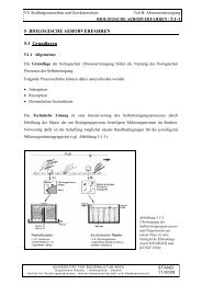
LAI detectionLAI = sum of the projected leaf surface persoil areaLAI = s/Gwhere: s is the projected leaf area (m 2 )G is the ground area (m 2 )It is a dynamic parameterLAI varies with• species composition;• annual mean temperature;• vegetative period length;• plant age;• soil fertility;• season.Control boxIt is used to describe foreststructure, wood biomass andphotosynthesisLeaf area and biomass may beestimated using diffuse lightaccording to Beer’s law:I = I 0 e -k k Ldetectorsensorefiltrocampo di vistaspecchiolenti-- Introduction - The data -Methodology -- Analysis -- Conclusions --

Airborne laser scanningLiDAR data were processed using Terrascansoftware ©Terrasolid, Finland. Ground pointswere filtered by an automatic procedure(Axelsson, 2000).Vegetation points were divided in two classes:- low vegetation (h ≤ 1 m above the ground);- high vegetation (h >1 m above the ground).g/v = 0.084 (spruce(forest)g/v = 0.035 (beech(forest)Indirect LAI measurements are based on solar lighttransmission or reflectance through vegetation.This can be assumed to be similar to the transmissionof the laser beam through the canopy.On the basis of this assumption, a Laser PenetrationIndex (LPI) was defined as follow:g ij = ground points densityLPI ij = g ij / (g(ij + v ij )v ij = high vegetation points density-- Introduction -- The data - Methodology - Analysis -- Conclusions --

LiDAR penetration index (LPI)g ijLPI ij= g ij/ (g ij+ v ij)• non-homogenous distribution of LiDAR samplingpoints in the areas studied;v ij5 m, appropriate for a 2 pts/m 2 sampling density.• g ij and v ij were assigned to each cell according to aneighbourhood statistical analysis using a radius of• g ij in the denominator allows the normalization oflocal variations of the sampling density due toLiDAR strips overlapping and variation of thehelicopter speed.-- Introduction -- The data - Methodology - Analysis -- Conclusions --

LiDAR penetration index (LPI)g ijLPI ij= g ij/ (g ij+ v ij)• non-homogenous distribution of LiDAR samplingpoints in the areas studied;v ij5 m, appropriate for a 2 pts/m 2 sampling density.• g ij and v ij were assigned to each cell according to aneighbourhood statistical analysis using a radius of• g ij in the denominator allows the normalization oflocal variations of the sampling density due toLiDAR strips overlapping and variation of thehelicopter speed.100 m-- Introduction -- The data - Methodology - Analysis -- Conclusions --

LiDAR penetration indexLPI values close to 0 describe a dense vegetationwhile values close to 1 are characteristic of an openstand or a clear ground.Automatic classification forest – non forest areas100 m-- Introduction -- The data --Methodology - Analysis - Conclusions --

LiDAR penetration indexLAI and LPI values for each plotTransect area m 2 forest_cat LAI mean_LPI1 400 spruce 3,73 0,162 400 spruce 3,8 0,133 400 spruce 3,83 0,134 400 spruce-fir 4,6 0,055 400 spruce-fir 4,56 0,066 400 spruce-fir 4,41 0,087 400 spruce-fir 4,27 0,078 400 spruce-fir 4,71 0,109 400 spruce-fir 4,13 0,1410 400 spruce 4,18 0,1411 400 spruce 3,54 0,1612 400 spruce 3,64 0,1513 10.000 spruce-fir 4,3 0,1314 10.000 spruce 3,21 0,1915 1.000 beech 5,78 0,0116 1.000 ash-mixed 5 0,0317 400 ash-mixed 5,42 0,0218 400 beech 5,69 0,0219 400 beech 5,42 0,0220 10.000 beech 5,49 0,02LPI values close to 0 describe a dense vegetationwhile values close to 1 are characteristic of an openstand or a clear ground.Automatic classification forest – non forest areasLAI = -12.86 * LPI + 5.59Linear regression analysis7,006,005,00Broaded leaf foresty = -12,863x + 5,5919R 2 = 0,89LAI4,003,002,00Coniferous forest1,000,000 0,02 0,04 0,06 0,08 0,1 0,12 0,14 0,16 0,18 0,2mean LPI100 m-- Introduction -- The data --Methodology - Analysis - Conclusions --

Data analysis• A random re-sampling procedure of LiDAR data to estimate different laser points densitieswas performed (from a density of 2 pts/m 2 to 1 pts/100 m 2 ).R 2 1,000,890,900,850,890,790,800,840,700,710,680,700,650,730,57 0,610,600,530,500,550,490,400,410,30Constant radius (5 m)0,20Variable radius0,260,27Polynomial interpolation0,210,100,110,002 1 0,5 0,25 0,12 0,05 0,028 0,02 0,013 0,01Points density (pts/m2)The pattern of correlation coefficient(R 2 ) between measured LAI and LPIcalculated on the basis ofneighbourhood analysis performedusing a fixed radius (5 m) is reportedin blue.In this case, R 2 decreases very fast byreducing laser points density.To have a constant number of sampling points, a variable radius for each re-sampling wasused applying the equation:r = (150/πρπρ) ½where r is in meters, ρ is the points density (pts/m 2 ) and 150 is the number of points with aradius of 5 m and a points density of 2 pts/m 2 .-- Introduction -- The data --Methodology - Analysis - Conclusions --

Data analysis• The variation of R 2 for the correlation between LPI and LAI at different points densities.7,007,007,006,00y = -12,863x + 5,5919R 2 = 0,896,00y = -10,927x + 5,5815R 2 = 0,856,00y = -9,4221x + 5,5271R 2 = 0,795,005,005,00LAI4,003,00LAI4,003,00LAI4,003,002,001,00LPI = 0.192,001,00LPI = 0.242,001,00LPI = 0.290,000 0,02 0,04 0,06 0,08 0,1 0,12 0,14 0,16 0,18 0,2mean LPI0,000,00 0,05 0,10 0,15 0,20 0,25 0,30mean LPI0,000,00 0,05 0,10 0,15 0,20 0,25 0,30 0,35mean LPI7,006,00y = -8,3121x + 5,4366R 2 = 0,707,006,00y = -7,5172x + 5,3531R 2 = 0,657,006,00y = -6,1567x + 5,3615R 2 = 0,685,005,005,00LAI4,003,00LAI4,003,00LAI4,003,002,001,00LPI = 0.332,001,00LPI = 0.382,001,00LPI = 0.450,000,00 0,05 0,10 0,15 0,20 0,25 0,30 0,35mean LPI0,000,00 0,05 0,10 0,15 0,20 0,25 0,30 0,35 0,40meanLPI0,000,00 0,05 0,10 0,15 0,20 0,25 0,30 0,35 0,40 0,45 0,50mean LPI7,006,005,00y = -5,5628x + 5,2786R 2 = 0,537,006,005,00y = -7,3055x + 5,6896R 2 = 0,717,006,005,00y = -7,2738x + 5,6629R 2 = 0,57LAI4,003,00LAI4,003,00LAI4,003,002,001,00LPI = 0.452,001,00LPI = 0.412,001,00LPI = 0.370,000,00 0,05 0,10 0,15 0,20 0,25 0,30 0,35 0,40 0,45 0,50mean LPI0,000,00 0,05 0,10 0,15 0,20 0,25 0,30 0,35 0,40 0,45mean LPI0,000,00 0,05 0,10 0,15 0,20 0,25 0,30 0,35 0,40mean LPI-- Introduction -- The data --Methodology - Analysis - Conclusions --

Data analysisPts/m2 2 – 1 – 0.5 – 0.25 – 0.12 – 0.05 – 0.028 – 0.02 – 0.013 – 0.01The variation of the spatial values of Laser Penetration Index usingdifferent sample density-- Introduction -- The data --Methodology - Analysis - Conclusions --

Conclusion• The significant linear correlationbetween field LAI values and LPI(R 2 =0.89, P

Thank you for yourattentionhttp://geomatica.uniud.ite.mail: : andrea.barilotti@uniud.it