9-3 laminar flat-plate boundary layer: exact solution - Université d ...

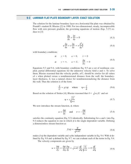
9-3 LAMINAR FLAT-PLATE BOUNDARY LAYER: EXACT SOLUTION S-399-3 LAMINAR FLAT-PLATE BOUNDARY LAYER: EXACT SOLUTIONThe solution for the laminar boundary layer on a horizontal flat plate was obtained byPrandtl’s student H. Blasius [2] in 1908. For two-dimensional, steady, incompressibleflow with zero pressure gradient, the governing equations of motion (Eqs. 5.27) reduceto [3]∂u∂ + ∂ vx ∂ y= 0(9.3)∂uu u u∂ x∂ y∂v 2∂y(9.4)with boundary conditionsat y 0, u 0, v 0at y , u U,∂u(9.5) 0∂yEquations 9.3 and 9.4, with boundary conditions Eq. 9.5 are a set of nonlinear, coupled,partial differential equations for the unknown velocity field u and v. To solvethem, Blasius reasoned that the velocity profile, u/U, should be similar for all valuesof x when plotted versus a nondimensional distance from the wall; the boundarylayerthickness, , was a natural choice for nondimensionalizing the distance fromthe wall. Thus the solution is of the formuy= g ( ) where ∝U(9.6)Based on the solution of Stokes [4], Blasius reasoned that xUand set2U = y xWe now introduce the stream function, , whereu = ∂ =− ∂ and v∂y ∂x(9.7)(5.4)satisfies the continuity equation (Eq. 9.3) identically. Substituting for u and v into Eq.9.4 reduces the equation to one in which is the single dependent variable. Defininga dimensionless stream function asf( )= xU(9.8)makes f() the dependent variable and the independent variable in Eq. 9.4. With definedby Eq. 9.8 and defined by Eq. 9.7, we can evaluate each of the terms in Eq. 9.4.The velocity components are given byuxU df U= ∂ = ∂ ∂= = U df∂y∂∂yd xd(9.9)

S-40 CHAPTER 9 / EXTERNAL INCOMPRESSIBLE VISCOUS FLOWandv =− ∂ ⎡=−⎢∂x⎣ xU∂ f ∂ x+12U⎤ ⎡⎥ =−⎢x f⎦ ⎣df ⎛ 1 1 xU − ⎞d⎝ 2 x⎠ + 12U⎤⎥x f⎦or1 U ⎡ df ⎤v = ⎢− f2 x ⎣ d ⎥⎦By differentiating the velocity components, it also can be shown thatand∂uU d f=− ∂x2xd 2∂u= U U x d 2f2∂ydSubstituting these expressions into Eq. 9.4, we obtain232 3d f3∂ u U2=∂y x d(9.10)d f23+ f d f2= 0(9.11)ddwith boundary conditions:dfat = 0, f = = 0ddfat →∞ , = 1(9.12)dThe second-order partial differential equations governing the growth of the laminarboundary layer on a flat plate (Eqs. 9.3 and 9.4) have been transformed to a nonlinear,third-order ordinary differential equation (Eq. 9.11) with boundary conditionsgiven by Eq. 9.12. It is not possible to solve Eq. 9.11 in closed form; Blasius solved itusing a power series expansion about 0 matched to an asymptotic expansion for : . The same equation later was solved more precisely—again using numericalmethods—by Howarth [5], who reported results to 5 decimal places. The numericalvalues of f, df/d, and d 2 f/d 2 in Table 9.1 were calculated with a personal computerusing 4th-order Runge-Kutta numerical integration.The velocity profile is obtained in dimensionless form by plotting u/U versus ,using values from Table 9.1. The resulting profile is sketched in Fig. 9.3b. Velocityprofiles measured experimentally are in excellent agreement with the analytical solution.Profiles from all locations on a flat plate are similar; they collapse to a singleprofile when plotted in nondimensional coordinates.From Table 9.1, we see that at 5.0, u/U 0.992. With the boundary-layerthickness, , defined as the value of y for which u/U 0.99, Eq. 9.7 gives2250 . 50 . x ≈ =U x Re x(9.13)

9-3 LAMINAR FLAT-PLATE BOUNDARY LAYER: EXACT SOLUTION S-41Table 9.1The Function f() for the Laminar Boundary Layer along a Flat Plate atZero Incidence = yUxff ′ =uUfThen0 0 0 0.33210.5 0.0415 0.1659 0.33091.0 0.1656 0.3298 0.32301.5 0.3701 0.4868 0.30262.0 0.6500 0.6298 0.26682.5 0.9963 0.7513 0.21743.0 1.3968 0.8460 0.16143.5 1.8377 0.9130 0.10784.0 2.3057 0.9555 0.06424.5 2.7901 0.9795 0.03405.0 3.2833 0.9915 0.01595.5 3.7806 0.9969 0.00666.0 4.2796 0.9990 0.00246.5 4.7793 0.9997 0.00087.0 5.2792 0.9999 0.00027.5 5.7792 1.0000 0.00018.0 6.2792 1.0000 0.0000The wall shear stress may be expressed as∂u⎤w U U x d f ⎤=∂y⎥ =2 ⎥⎦d⎦y= 0 = 02w= 0.332UU x =0.332URex2(9.14)and the wall shear stress coefficient, C f , is given byCf w=2=U120.664Rex(9.15)EXAMPLE 9.2Each of the results for boundary-layer thickness, , wall shear stress, w , andskin friction coefficient, C f , Eqs. 9.13 through 9.15, depends on the length Reynoldsnumber, Re x , to the one-half power. The boundary-layer thickness increases as x 1/2 ,and the wall shear stress and skin friction coefficient vary as 1/x 1/2 . These resultscharacterize the behavior of the laminar boundary layer on a flat plate.Laminar Boundary Layer on a Flat Plate: Exact SolutionUse the numerical results presented in Table 9.1 to evaluate the following quantitiesfor laminar boundary-layer flow on a flat plate:(a) */ (for 5 and as : ).(b) v/U at the boundary-layer edge.(c) Ratio of the slope of a streamline at the boundary-layer edge to the slope of versus x.

S-42 CHAPTER 9 / EXTERNAL INCOMPRESSIBLE VISCOUS FLOWEXAMPLE PROBLEM 9.2GIVEN: Numerical solution for laminar flat-plate boundary layer, Table 9.1.FIND:(a) * / (for 5 and as : ).(b) v/U at boundary-layer edge.(c) Ratio of the slope of a streamline at the boundary-layer edge to the slope of versus x.SOLUTION:The displacement thickness is defined by Eq. 9.1 as* =⎛−⎞≈⎛−⎞∫ ∞ u1 10 ⎝ U ⎠dy u∫0⎝ U ⎠dyIn order to use the Blasius exact solution to evaluate this integral, we need to convert it from one involving u andUy to one involving f ( u/U) and variables. From Eq. 9.7, x x= y , so y = and dy = d xUUThus, * max xmax= ( 1− f ) = ( 1−) (1)∫0 U d xfdU ∫0Note: Corresponding to the upper limit on y in Eq. 9.1, max , or max 5.From Eq. 9.13,5 ≈U xso if we divide each side of Eq. 1 by each side of Eq. 9.13, we obtain (with f df/d)1 ⎛ df ⎞= ⎜1− ⎟ d5 ∫0⎝ d⎠* maxIntegrating givesEvaluating at max 5, we obtain * 1= [ − f ( ) ]max50The quantity f() becomes constant for 7. Evaluating at max 8 gives*Thus, * : is 0.24 percent larger than * 5 From Eq. 9.10,*1* = ( 5. 0 − 3. 2833) = 0.343 ( = 5 )5 ←⎯⎯⎯⎯⎯⎯⎯⎯⎯⎯⎯⎯⎯⎯⎯⎯1= (. 8 0 − 6. 2792) = 0.3445*( →∞)←⎯⎯⎯⎯⎯⎯⎯⎯⎯⎯⎯⎯⎯ ⎯⎯1 U⎛ df ⎞ vv = ⎜ −⎝ ⎠⎟ = 1 ⎛ df⎜⎝− ⎞ 1 ⎛ df f , so f ⎟ = ⎜ −2 x d U 2 Ux d ⎠ 2 Re ⎝ d x⎞f ⎟⎠

9-3 LAMINAR FLAT-PLATE BOUNDARY LAYER: EXACT SOLUTION S-43Evaluating at the boundary-layer edge ( 5), we obtainv 10. 837 0.84v= [(. 5 0 9915) − 3. 2833]= ≈ ( = 5)U 2 Rex Rex Rex←⎯⎯⎯⎯⎯⎯⎯⎯⎯⎯⎯U ⎯Thus v is only 0.84 percent of U at Re x 10 4 , and only about 0.12 percent of U at Re x 5 10 5 .The slope of a streamline at the boundary-layer edge isdy⎞v v 084 .= = ≈dx ⎠streamline u U Re xThe slope of the boundary-layer edge may be obtained from Eq. 9.13,so5 ≈ = 5U x xUd 1 −12= 5 x = 25 . =dx U 2Ux25 .Re xdyThus⎞dx ⎠streamline084 . dddy⎞= = 0.33625 . dx dxdx ⎠streamline←⎯⎯⎯⎯⎯⎯⎯⎯⎯⎯⎯⎯⎯⎯⎯⎯⎯⎯⎯⎯⎯⎯This result indicates that the slope of the streamlines is about 1/3 of the slope of the boundary layeredge—the streamlines penetrate the boundary layer, as sketched below:UUuδThis problem illustrates use of numerical data from the Blasiussolution to obtain other information on a flat plate laminarboundary layer, including the result that the edge of theboundary layer is not a streamline.