Paper

More documents

Recommendations

Info

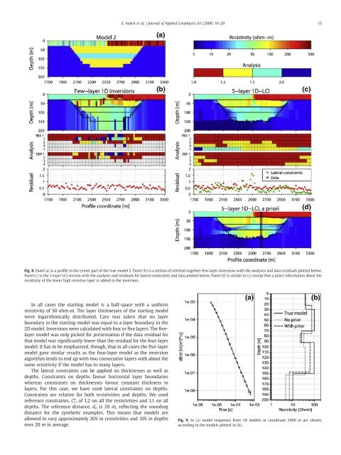
E. Auken et al. / Journal of Applied Geophysics 65 (2008) 10–2015Fig. 8. Panel (a) is a profile in the center part of the true model 2. Panel (b) is a section of stitched-together few-layer inversions with the analyses and data residuals plotted below.Panel (c) is the 5-layer LCI-section with the analyses and residuals for lateral constraints and data plotted below. Panel (d) is similar to (c) except that a priori information about theresistivity of the lower high-resistive layer is added to the inversion.In all cases the starting model is a half-space with a uniformresistivity of 50 ohm-m. The layer thicknesses of the starting modelwere logarithmically distributed. Care was taken that no layerboundary in the starting model was equal to a layer boundary in the2D model. Inversions were calculated with four or five layers. The fivelayermodel was only picked for presentation if the data residual forthat model was significantly lower than the residual for the four-layermodel. It has to be emphasised, though, that in all cases the five-layermodel gave similar results as the four-layer model as the inversionalgorithm tends to end up with two consecutive layers with about thesame resistivity if the model has to many layers.The lateral constraints can be applied on thicknesses as well asdepths. Constraints on depths favour horizontal layer boundarieswhereas constraints on thicknesses favour constant thickness inlayers. For this case, we have used lateral constraints on depths.Constraints are relative for both resistivities and depths. We usedreference constraints, C r n , of 1.2 on all the resistivities and 1.1 on alldepths. The reference distance, d r ,is20m,reflecting the soundingdistance for the synthetic examples. This means that models areallowed to vary approximately 20% in resistivities and 10% in depthsover 20 m in average.Fig. 9. In (a) model responses from 1D models at coordinate 2400 m are shown,according to the models plotted in (b).
16 E. Auken et al. / Journal of Applied Geophysics 65 (2008) 10–203.1. Model 1 — simple incised valleyThe first synthetic model shown in Fig. 6a is a simple incised valleywith a varying cover layer.The few-layer stitched-together model section is presented in Fig. 6b.The top-layer is well resolved in both sides, with mean resistivitiesreflecting the mean resistivities of the layer. The resistivity change in thecentral part is also resolved, with only an indication of associated 2Deffects. On the flanks of the valley, the high-resistive bottom layer isresolved, but in the central part, for depths larger than 130 m, the bottomlayer cannot be resolved. The parameter analyses reflect mainly welldetermined parameters whenever the model has only two layers and asomewhat poorer determination of the three- and four-layer models.The data residuals are in all cases well below one, indicating that data arefitted within the observation error.A four-layer LCI model is shown in Fig. 6c. The most pronounceddifference compared to the few-layer inversion is the resolution of thedepth of the valley for the entire profile. The lateral constraints drawinformation on the layer boundaries and layer resistivities to thecentre of the profile, where only limited information of the depth tothe bottom of the valley is available. The analyses present well tomoderately-well determined parameters. The depth to the bottom ofthe valley is well determined taking advantage of the informationcoming from the lateral constraints. The data residuals of the lateralconstraints are well below one, except for the central part where thelateral constraints are “stressed” due to the rapid resistivity changes inthe first layer required by the data.Fig. 7 shows plotted data and models from coordinate 2400.Obviously there is little evidence in the data about the bottom layer atthis position as reflected in the few-layer inversions. However,including the lateral constraints restricting the geological variationwe see that the resulting model closely resembles that of the true 1Dmodel at that site. The underestimated depth to the bottom layer ismost likely explained by 2D effects from the sides of the valley causingthe signal to be too low at late times.3.2. Model 2 — low-resistive layerThe valley model in Fig. 8a is incised in a low-resistivity backgroundwith a high-resistivity fill containing a low-resistivity layer.The few-layer stitched-together model section is presented inFig. 8b. Similar to the analysis of model 1, the top-layer is well resolvedFig. 10. Panel (a) is a profile in the center part of the true model 4. Panel (b) is a section of stitched-together few-layer inversions with the analyses and data residuals plotted below.Panel (c) is the 5-layer LCI-section with the analyses and residuals for lateral constraints and data plotted below. Panel (d) is a section of stitched-together few-layer inversions withthe magnetic moment increased to 50,000 Am 2 . Panel (e) is the 5-layer LCI-section obtained with the high-moment data. The analyses use a 4-graded color code ranging from red(well determined) to blue (undetermined).
Page 4 and 5: E. Auken et al. / Journal of Applie

Paper

You also want an ePaper? Increase the reach of your titles

Delete template?

Save as template?