guideline and standards for skytem measurements, processing and ...
guideline and standards for skytem measurements, processing and ...
guideline and standards for skytem measurements, processing and ...

You also want an ePaper? Increase the reach of your titles
YUMPU automatically turns print PDFs into web optimized ePapers that Google loves.
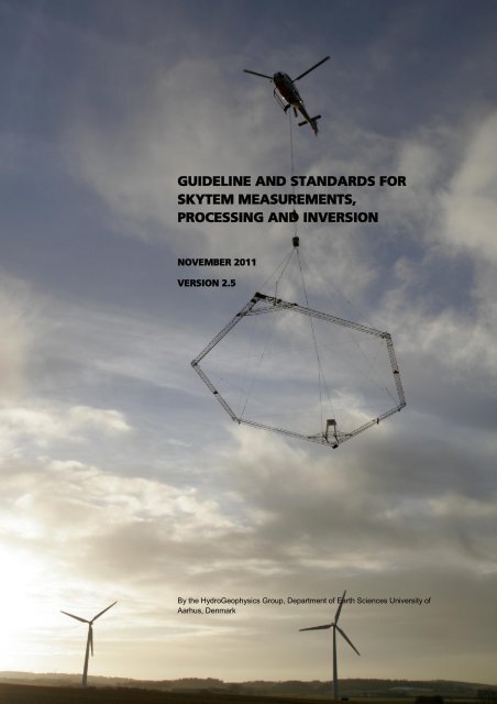
GUIDELINE AND STANDARDS FOR<br />
SKYTEM MEASUREMENTS,<br />
PROCESSING AND INVERSION<br />
NOVEMBER 2011<br />
VERSION 2.5<br />
By the HydroGeophysics Group, Department of Earth Sciences University of<br />
Aarhus, Denmark<br />
1
TABLE OF CONTENTS<br />
1 Revision history ................................................................................ 3<br />
2 Introduction ....................................................................................... 5<br />
3 SkyTEM configuration <strong>and</strong> measurement strategies ..................... 6<br />
3.1 SkyTEM configurations ........................................................................... 6<br />
3.2 Flight lines................................................................................................ 7<br />
3.3 Flight speed, altitude <strong>and</strong> frame angle ................................................... 7<br />
4 Validation procedures ....................................................................... 9<br />
4.1 Calibration – National test site Aarhus ................................................... 9<br />
4.2 Determination of transmitter wave<strong>for</strong>m .................................................. 9<br />
4.3 Local reference locality ........................................................................... 11<br />
4.4 Bias test during production flight ............................................................ 11<br />
4.5 Measurements at high altitude - system response determination ........ 12<br />
5 Data reporting .................................................................................... 13<br />
5.1 SkyTEM ApS reporting ........................................................................... 17<br />
6 Data <strong>processing</strong> ................................................................................ 19<br />
6.1 Assessment in connection with data <strong>processing</strong> ................................... 19<br />
6.2 GPS, angle <strong>and</strong> altitude data.................................................................. 20<br />
6.3 db/dt data ................................................................................................. 20<br />
6.4 Coupled data ........................................................................................... 21<br />
6.5 Averaging <strong>and</strong> trimming of data ............................................................. 22<br />
7 Data Inversion.................................................................................... 24<br />
7.1 Assessment in connection with data inversion ...................................... 24<br />
7.2 Inversion model ....................................................................................... 25<br />
7.3 Constrained Inversion ............................................................................. 26<br />
7.4 SCI ........................................................................................................... 27<br />
7.5 Inversion workflow ................................................................................... 27<br />
8 Reporting on <strong>processing</strong> <strong>and</strong> inversion .......................................... 29<br />
8.1 Processing ............................................................................................... 29<br />
8.2 Inversion results ...................................................................................... 29<br />
8.3 Reporting, GERDA .................................................................................. 29<br />
9 References ......................................................................................... 30<br />
2
1 REVISION HISTORY<br />
This <strong>guideline</strong> has been updated <strong>and</strong> revised repeatedly. In the following, we<br />
summarize the main revisions made.<br />
Version 1.1<br />
Changes to averaging filter widths.<br />
Minor changes made in the <strong>processing</strong> section, including averaging filter widths.<br />
Minor changes made in the inversion section, including recommended model<br />
setup.<br />
Specification of the repetition frequency in the raw data report.<br />
Version 2.0<br />
The <strong>guideline</strong> was thoroughly revised <strong>and</strong> restructured. The <strong>guideline</strong> was<br />
amended to reflect the currently used SkyTEM equipment including updated<br />
specifications <strong>and</strong> method & data collection requirements. The <strong>processing</strong> <strong>and</strong><br />
inversion sections were exp<strong>and</strong>ed <strong>and</strong> updated.<br />
Furthermore, based on experiences with the previous <strong>guideline</strong> <strong>and</strong> per<strong>for</strong>med<br />
SkyTEM mappings, a number of details were clarified concerning data<br />
collection, <strong>processing</strong>, inversion <strong>and</strong> reporting of mappings.<br />
Main changes <strong>and</strong> amendments to the current version:<br />
A description of the various SkyTEM setups <strong>and</strong> their uses was added to the<br />
manual<br />
In a number of places, text <strong>and</strong> sections were reorganized slightly to achieve<br />
a more consistent presentation<br />
Sections on calibration including bias <strong>and</strong> altitude testing were added<br />
New sections were added on line numbering <strong>and</strong> positioning of flight lines.<br />
Requirements <strong>for</strong> the <strong>processing</strong> <strong>and</strong> inversion of SkyTEM data were<br />
described<br />
Appendices with detailed SkyTEM setup options <strong>and</strong> <strong>processing</strong> <strong>and</strong> inversion<br />
system settings were added<br />
The SkyTEM file <strong>for</strong>mats were documented.<br />
The changes are so comprehensive that the manual was presented to all<br />
interested parties at a meeting in January 2010.<br />
Version 2.1 – 5 August 2010<br />
A new appendix was added to this version - Appendix 7 - comprising a detailed<br />
description of the st<strong>and</strong>ard map types included in data reports. References to<br />
the new appendix were added to section 8.2.<br />
Version 2.3 – December 2010<br />
Extension of appendix 5 with SCI-settings<br />
Minor changes on pages 22, paragraph ”noise <strong>processing</strong> “<br />
Appendix 1 SkyTEM-setup: The gate width <strong>for</strong> time gate in the interval 6s to<br />
13 s SLM is chanced resulting in more robust gates.<br />
Version 2.4 – January 2011<br />
A new setting <strong>for</strong> the <strong>processing</strong> of the GPS-data in Aarhus Workbench is<br />
added. This setting enables the user to shift the GPS-position in flight direction<br />
to obtain the optimum geographical positions <strong>for</strong> the data/models. Appendix 4.<br />
has been updated with this setting inc. comments <strong>and</strong> recommended values.<br />
The inversion code em1dinv has been updated to h<strong>and</strong>le larger LCIsections/SCI-cells.<br />
Recommended LCI-sections/SCI-cells sizes have there<strong>for</strong>e<br />
been updated in Appendix 5.<br />
3
Version 2.5 – November 2011<br />
In chapter 4.1 it is now specified that the calibration has to be per<strong>for</strong>med with<br />
the refined national TEM reference model from Aarhus testsite.<br />
Minor corrections in Appendix 3. , regarding the geometry file.<br />
4
2 INTRODUCTION<br />
This report is a translation of the Danish version of the “Guideline <strong>and</strong> st<strong>and</strong>ards<br />
<strong>for</strong> SkyTEM <strong>measurements</strong>, <strong>processing</strong> <strong>and</strong> inversion”. The intention is to keep<br />
the English version up-to-date with the Danish version. The Danish version is<br />
valid <strong>for</strong> the partners involved in SkyTEM surveys in Denmark.<br />
The helicopter-borne transient electromagnetic measurement method, SkyTEM,<br />
is the leading geophysical method used <strong>for</strong> groundwater mapping in Denmark.<br />
This <strong>guideline</strong> was made as a quality assurance measure to ensure the quality<br />
of the procedures per<strong>for</strong>med during SkyTEM data collection <strong>and</strong> <strong>processing</strong>.<br />
The st<strong>and</strong>ards presented herein are tailored to Danish geological conditions <strong>and</strong><br />
to local Danish requirements concerning data quality <strong>and</strong> inversion.<br />
The manual is comprised by two main sections: Data collection, validation <strong>and</strong><br />
documentation are detailed in sections 3-5. Processing, inversion <strong>and</strong> reporting<br />
to GERDA are described in sections 6-8. Furthermore, the manual contains a<br />
number of appendices detailing various instrumentation <strong>and</strong> <strong>processing</strong><br />
parameters. These appendices may be useful in connection with the drafting of<br />
agreements.<br />
As the measurement equipment <strong>and</strong> inversion software are improved over time,<br />
the manual will be updated, as needed.<br />
The requirements to field work <strong>and</strong> data <strong>processing</strong> presented in the manual are<br />
st<strong>and</strong>ard requirements. In case these requirements cannot be met, the reasons<br />
<strong>for</strong> this shall be stated clearly in the final report <strong>and</strong>, where relevant, the involved<br />
parties shall be in<strong>for</strong>med. The <strong>guideline</strong> also provides a number of<br />
recommended <strong>processing</strong> <strong>and</strong> inversion settings.<br />
The <strong>guideline</strong> was circulated <strong>for</strong> comment in GEUS <strong>and</strong> among consulting<br />
engineers. All interested parties were invited to a meeting held at the<br />
Department of Earth Sciences in January 2010.<br />
Please note that the percentages provided in section 4.3 are presently<br />
instructive only. Final determination of the percentages presupposes thorough<br />
investigation.<br />
Version 2.0 of the manual came into <strong>for</strong>ce on 15 February 2010. The newest<br />
version is available from the web page of the HydroGeophysics Group:<br />
www.gfs.au.dk<br />
5
3 SKYTEM CONFIGURATION AND MEASUREMENT<br />
STRATEGIES<br />
Below we present the various SkyTEM configurations, positioning of flight lines<br />
<strong>and</strong> determination of flight speed <strong>and</strong> altitude. The SkyTEM method is also<br />
described in ref. /8/.<br />
3.1 SkyTEM configurations<br />
Generally, the SkyTEM system measurement configuration needs to be<br />
adjusted to fit the mapping area <strong>and</strong> purpose. The system may be adjusted in a<br />
number of ways to facilitate mapping of very surface-near geological structures,<br />
profound structures or intermediary layers. Appendix 1 comprises a number of<br />
st<strong>and</strong>ard configurations, optimized <strong>for</strong> each of the mentioned mapping<br />
purposes.<br />
The system uses a combination of two moments, super low moment (SLM) <strong>and</strong><br />
high moment (HM). Previous versions of the SkyTEM also used low moment<br />
(LM). This is not currently the case, as LM was replaced by SLM. The SLM <strong>and</strong><br />
HM have the following characteristics:<br />
Super low moment (SLM)<br />
One turn is employed on the transmitter frame, <strong>and</strong> a current of approx. 10 A is<br />
used. The first usable gate time depends on the choice of HM <strong>and</strong> is<br />
somewhere in the 10-15 ìs interval. SLM yields maximum resolution of surfacenear<br />
geological structures.<br />
High moment (HM)<br />
The maximum transmitter current is 110 A in 1 to 4 turns. The first usable gate<br />
time occurs at approx. 30-70 ìs. Two frame sizes are available, measuring<br />
approx. 314 m 2 <strong>and</strong> 494 m 2 . When the smaller frame is used, configurations with<br />
1 (HM1), 2 (HM2) or 4 (HM4) turns are possible. If the larger frame is employed,<br />
four turns are always used.<br />
The larger frame is mainly used <strong>for</strong> mappings requiring a substantial mapping<br />
depth (up to 300 m), while the smaller frame is used where mapping depths of<br />
up to 200 m are needed. If HM1 <strong>and</strong> HM2 are used, the mapping depth is more<br />
limited (100-150 m) as <strong>measurements</strong> are limited to 1.2-4 ms (versus the normal<br />
10 ms) period.<br />
In two or four turn configurations, SLM will not yield as early gate times as when<br />
using one turn with a single turn.<br />
Moment combinations <strong>and</strong> lateral resolution<br />
SLM in combination with HM1 <strong>and</strong> HM2 yield a very dense lateral data sampling<br />
resulting in a very high resolution of surface-near geology. By combining SLM<br />
<strong>and</strong> HM4, considerable mapping depth is achieved, but as transmission occurs<br />
at a lower frequency <strong>and</strong> over a longer period of time, lateral data sampling is<br />
less dense <strong>and</strong> the geology of very surface-near there<strong>for</strong>e somewhat limited.<br />
For approx. every 20 th shift of moment, the HM background noise is measured<br />
at a reduced stack size. This measurement is used during <strong>processing</strong> to assess<br />
the noise.<br />
6
3.2 Flight lines<br />
Generally, the positioning of flight lines is agreed upon by SkyTEM ApS <strong>and</strong> the<br />
client.<br />
Flight line positioning<br />
Lateral resolution will always be greater along the flight lines than<br />
perpendicularly to these. Normally, it will there<strong>for</strong>e be beneficial to place the<br />
lines so that they cross any known/expected geological structures. Wind <strong>and</strong><br />
weather conditions experienced while mapping may affect the orientation of<br />
flight lines. However, at higher line densities, the impact of line orientation on<br />
mapping results is more limited.<br />
Flight lines are positioned as straight lines. Lines which run along ground<br />
installations over long distances <strong>and</strong> at a distance not exceeding 100 m are not<br />
measured as they result in coupled data. However, the distance depends on the<br />
specific geology, as a high resistivity in the upper layers will entail a need <strong>for</strong><br />
further distance to any installations. Experience shows that a distance of the<br />
above-mentioned 100 m is needed at resistivities ranging from 30 to 80 Ùm,<br />
while the distance needed at resistivities above 200-300 Ùm may exceed 200<br />
m.<br />
The actual flight lines may deviate somewhat from the planned straight flight<br />
lines, as the actual route taken is decided by the helicopter pilot in accordance<br />
with safety considerations. For instance, the pilot will need to avoid buildings<br />
<strong>and</strong> some types of farm animals, tall trees <strong>and</strong> high-voltage power lines.<br />
Placing flight lines at short intervals will provide a high lateral resolution of the<br />
geological layers. A maximum line distance of 200 m (5 line kilometres per km 2 )<br />
when a large mapping depth is a priority, <strong>and</strong> approx. 170 m (6 line kilometres<br />
per km 2 ) when structures nearer to the surface are to be mapped. In special<br />
priority areas, it may be relevant to reduce line distance to as little as 50 m.<br />
3.3 Flight speed, altitude <strong>and</strong> frame angle<br />
Flight speed<br />
The selected flight speed is a trade-off between lateral resolution, mapping<br />
depth <strong>and</strong> costs. A low speed leads to a high data density, which results in an<br />
improved lateral resolution <strong>and</strong> a higher mapping depth.<br />
Generally, flight speed should be maintained as constant as possible. Major<br />
speed fluctuations over short distances distort subsequent data <strong>processing</strong> with<br />
regard to mapping depth <strong>and</strong> lateral resolution. The flight speed target should be<br />
45 km/t (12,5 m/s) <strong>and</strong> fluctuations to above 55 km/t <strong>for</strong> more than a few<br />
consecutive minutes should be avoided. If the flight speed/average speed<br />
deviates from what was agreed, this requires the acceptance of the client. Given<br />
the current system configurations, the stated flight speed is considered optimal<br />
<strong>for</strong> Danish conditions.<br />
Flight altitude<br />
The flight altitude has considerable impact on the size of the ground response,<br />
particularly in early time <strong>measurements</strong>. All things equal, the signal-to-noise<br />
ratio will be lower at low altitudes. For reasons of safety, the target altitude in<br />
open terrain is approx. 30 m, with fluctuations ranging from 25 to 45 m. Over<br />
7
woodl<strong>and</strong> <strong>and</strong> installations, the altitude is increased by the height of the objects<br />
overflown.<br />
Generally, the altitude should be maintained as low <strong>and</strong> as constant as possible.<br />
Major altitude fluctuations over short distances cause erroneous data<br />
<strong>processing</strong> <strong>and</strong> in some cases data must be discarded completely.<br />
Frame angle<br />
The frame should be maintained as horizontally as possible during flight. In<br />
practice, the frame cannot be maintained completely horizontal due to shifting<br />
winds <strong>and</strong> changes in flight direction <strong>and</strong> speed. Whenever possible, the frame<br />
should be suspended in such a manner that the angles (pitch <strong>and</strong> roll) do not<br />
exceed +/- 10 degrees in production scenarios. Angles exceeding 20 degrees in<br />
periods of less than 20 s are acceptable.<br />
8
4 VALIDATION PROCEDURES<br />
This section describes the validation procedures <strong>for</strong> SkyTEM equipment in<br />
connection with mapping.<br />
During any validation procedure, the SkyTEM system shall be configured as in<br />
the corresponding production scenario. The client shall be in<strong>for</strong>med of any<br />
configuration changes <strong>and</strong> of their influence on the validation of the equipment.<br />
If changes are significant, the equipment shall be revalidated.<br />
4.1 Calibration – National test site Aarhus<br />
The objective of calibrating the SkyTEM system at the National test site near<br />
Aarhus is to establish the absolute data level to facilitate precise data modelling.<br />
In connection with adaptation of the instruments, calibration <strong>measurements</strong> are<br />
always per<strong>for</strong>med. Furthermore, calibration <strong>measurements</strong> shall have been<br />
per<strong>for</strong>med three months or less be<strong>for</strong>e any mapping. The calibration has to be<br />
done with the refined TEM reference model from the National test site, as stated<br />
in /11/<br />
Determination of any time or level displacement is established by comparing a<br />
measured SkyTEM response to the <strong>for</strong>ward response from the geophysical<br />
ground model at the Aarhus test site. This is done <strong>for</strong> a minimum of three<br />
altitudes, typically approx. 10, 20 <strong>and</strong> 30 m. The <strong>for</strong>ward responses are<br />
calculated on the basis of the actual altitude <strong>and</strong> the entire SkyTEM system<br />
(transmitter wave<strong>for</strong>m, filters, front gate, etc.) is modelled. Thus, the wave<strong>for</strong>m<br />
shall be determined prior to the calculation of <strong>for</strong>ward responses. If the<br />
wave<strong>for</strong>m is altered, new <strong>for</strong>ward responses shall be generated <strong>and</strong> used <strong>for</strong><br />
calculation of calibration constants. This procedure is known as upward<br />
continuation.<br />
Documentation of the calibration is provided in the <strong>for</strong>m of a plot showing the<br />
<strong>for</strong>ward data <strong>and</strong> the measured data at the selected altitudes. A frame angle of<br />
approx. 0 degrees is the target. If the angle differs significantly from 0 degrees,<br />
adjustments should be made. The determined calibration constants should be<br />
identical <strong>for</strong> all measured altitudes.<br />
The difference between an upward continued <strong>for</strong>ward response <strong>for</strong> the model<br />
from the Aarhus test site <strong>and</strong> the measured response at every altitude shall not<br />
exceed 5% (rhoa data trans<strong>for</strong>mation) <strong>for</strong> data with a low noise level. Any<br />
deviations from this shall be presented to <strong>and</strong> accepted by the client.<br />
Please refer to /10/ <strong>for</strong> a general description of the calibration procedure.<br />
4.2 Determination of transmitter wave<strong>for</strong>m<br />
The objective of determining the transmitter wave<strong>for</strong>m is to enable precise<br />
modelling of the measured data.<br />
The transmitter wave<strong>for</strong>m consists of a turn-on ramp <strong>and</strong> a turn-off ramp. Turnon<br />
current is measured directly at the transmitter coil. The turn-off is measured<br />
9
as the time derivative of the current. When the wave<strong>for</strong>m is determined, the<br />
transmitter current shall have the same level as during production <strong>for</strong> the various<br />
moments. The wave<strong>for</strong>m shall be scalable to the transmitter current because<br />
minor wave<strong>for</strong>m fluctuations may occur during mapping, primarily due to<br />
temperature changes.<br />
The turn-on ramp is defined in the geometry file by an exponential function <strong>and</strong><br />
by placing “elbows” as shown in the upper half of Figure 1. The turn-off ramp is<br />
stated as a turn-off constant (A/s) <strong>for</strong> the linear avalanche process <strong>and</strong> an<br />
exponential constant <strong>for</strong> the free exponential decay (lower half of Figure 1). In<br />
the <strong>processing</strong> module of the Aarhus Workbench, the wave<strong>for</strong>m constants from<br />
the geometry file are translated into straight line subsections describing turn-on<br />
<strong>and</strong> turn-off ramps, as shown by the straight lines in Figure 1.<br />
Avalanche<br />
Exp. decay<br />
Figure 1. The figure shows the transmitter wave<strong>for</strong>m <strong>and</strong> how the <strong>for</strong>m is<br />
modelled in the Aarhus Workbench. Top - Turn-on ramp. The blue curve shows<br />
the measured current. The red curve shows the fitted exponential function<br />
(stated in the geometry file). The green line segments show the ramp used <strong>for</strong><br />
inversion. These are calculated using the exponential constant <strong>and</strong> the relevant<br />
transmitter current. Bottom - Turn-off ramp. The blue curve shows the measured<br />
integrated turn-off currents. The green line segments show the ramp used <strong>for</strong><br />
inversion. These are calculated using the exponential constant of the avalanche<br />
process, the exponential constant <strong>and</strong> the measured transmitter current.<br />
The determination of the wave<strong>for</strong>m is documented in the raw data report as a<br />
plot showing:<br />
The measured current data from the turn-on ramp with the selected<br />
exponential function<br />
10
The turn-off current with the selected exponential function. As data from the<br />
pick-up coil provides the time derivative of the actual current in the transmitter<br />
coil, a time-specific integration is per<strong>for</strong>med to determine the parameters of<br />
the avalanche process <strong>and</strong> the exponential decay process.<br />
Please refer to /4/ <strong>for</strong> a general description of the wave<strong>for</strong>m calculation.<br />
4.3 Local reference locality<br />
The objective of testing at the local reference locality is to ensure that the<br />
system remains error-free after mobilization <strong>and</strong> mapping.<br />
The local reference locality is established by per<strong>for</strong>ming five soundings using<br />
ground-based equipment. Be<strong>for</strong>e the soundings, this equipment shall have been<br />
calibrated at the Aarhus test locality. The soundings are per<strong>for</strong>med as a cross<br />
by placing the centres of each set-up at 40 m- intervals, as shown in<br />
Figure 2<br />
During the actual collection of production data - in connection with every flight<br />
<strong>and</strong> return flight - an approx. 30-second measurement should be per<strong>for</strong>med at<br />
the local reference locality with the frame located at production altitude. By<br />
comparing these <strong>measurements</strong>, the repeatability of data is documented.<br />
Furthermore, by comparing the <strong>measurements</strong> to the ground-based<br />
<strong>measurements</strong>, data reproducibility is also documented.<br />
The repeatability of all curves shall fall within 5% of the average value of every<br />
single gate (rhoa data trans<strong>for</strong>mation). The reproducibility of upward continued<br />
data from the ground model shall fall within 10% of the average value of every<br />
gate (rhoa data trans<strong>for</strong>mation). Both conditions apply to gates with a high<br />
signal-to-noise ratio. Any deviations from this shall be presented to <strong>and</strong><br />
accepted by the client.<br />
Figure 2. The local reference locality consists of five soundings with 40 m<br />
between the centres of each set-up.<br />
4.4 Bias test during production flight<br />
The objective of the bias test is to establish the bias level of early time<br />
<strong>measurements</strong> to facilitate the removal of any biased data. To establish any<br />
11
changes in the bias response, access flights as well as return flights shall reach<br />
an altitude of min. 300 m or as high as the cloud cover permits. Such altitude<br />
should be maintained <strong>for</strong> a minimum of 15 seconds.<br />
4.5 Measurements at high altitude - system response<br />
determination<br />
The objective of the altitude test is to identify the system response. The altitude<br />
test is per<strong>for</strong>med by measuring at an altitude at which the ground response is<br />
negligible, normally at approx. 1,000 m. One altitude test is per<strong>for</strong>med in<br />
connection with every mapping <strong>and</strong> in close proximity to or within the mapped<br />
area.<br />
The system response may not exceed approx. 2% (db/dt) of the ground<br />
response from the local reference locality at the normal production altitude. The<br />
size of the system response is documented in the <strong>for</strong>m of combined plots<br />
showing data (db/dt) from a high altitude <strong>and</strong> data from the normal production<br />
altitude. A large stack size shall be used <strong>for</strong> the db/dt data collected at high<br />
altitude to eliminate r<strong>and</strong>om background noise <strong>and</strong> ensure that the system<br />
response is clearly discernible. On the background hereof, SkyTEM ApS shall<br />
state in the geometry file which gate times are applicable.<br />
12
5 DATA REPORTING<br />
The SkyTEM system produces various data files. The next sections describe the<br />
data types <strong>and</strong> requirements related to raw data reporting. Furthermore, the<br />
SkyTEM equipment calibration requirements are outlined.<br />
The below section lists the instruments which collect the data that are<br />
subsequently processed <strong>and</strong> inversed. Figure 3 shows where the instruments<br />
are mounted.<br />
Data types<br />
SkyTEM shall supply all relevant data in accordance with the <strong>for</strong>mats <strong>and</strong><br />
conventions outlined below. Data shall be h<strong>and</strong>ed over as one comprehensive<br />
package.<br />
The data recorded during SkyTEM mapping shall be reported in the following file<br />
<strong>for</strong>mats:<br />
Geometry file<br />
SKB files<br />
SPS files<br />
Line number file<br />
Geometry file<br />
The geometry file contains in<strong>for</strong>mation on the configuration of the SkyTEM<br />
system. This in<strong>for</strong>mation is used during data <strong>processing</strong> <strong>and</strong> inversion. The<br />
geometry file is loaded with the remaining data to the Aarhus Workbench. It is a<br />
requirement that the final geometry file is h<strong>and</strong>ed-in along with the remaining<br />
data. A complete description of the geometry file is provided in Appendix 3. .<br />
The geometry file contains in<strong>for</strong>mation on:<br />
The placement of the various devices on the transmitter frame. The<br />
convention used <strong>for</strong> the system of coordinates is shown in Figure 3<br />
The expected transmitter current. Any deviation from the actually applied<br />
current may not exceed 25% of the expected transmitter current<br />
Size of the transmitter coil, number of turns <strong>and</strong> area covered<br />
Calibration constants in the <strong>for</strong>m of time <strong>and</strong> db/dt factors <strong>and</strong> constants<br />
Specification of the first usable gates of each channel<br />
Low-pass filters<br />
The front gate's position in time. The front gate shall occur a minimum of 1 ìs<br />
be<strong>for</strong>e the first usable gate opens<br />
The estimated attenuation of the primary field from the zero position<br />
Repetition frequency. Note that the repetition frequency stated in the<br />
geometry file is calculated as: RepetitionFrequencyGeo = 1/(4 x OnTime)<br />
Parameters describing the wave<strong>for</strong>m (turn-on <strong>and</strong> turn-off process) the turnoff<br />
process must be terminated be<strong>for</strong>e the front gate time (as stated above).<br />
Uni<strong>for</strong>m data STD. As st<strong>and</strong>ard 3% is used<br />
Gate centre times, gate factors, <strong>and</strong> gate opening <strong>and</strong> closing times.<br />
13
Figure 3. Sketch of the SkyTEM frame from above with indication of the primary<br />
instruments <strong>and</strong> definition of x <strong>and</strong> y directions. The x axis is the flight direction,<br />
the Y axis points to the right, <strong>and</strong> the Z axis points into the page.<br />
SPS files<br />
The SPS files contain:<br />
GPS data<br />
Pitch <strong>and</strong> roll (angle data)<br />
Altitude data<br />
Transmitter data, including transmitter current<br />
The instruments used to measure these data are all duplicated (except <strong>for</strong> the<br />
transmitter). Where possible, data from both instruments should be used.<br />
However, when only one of the duplicated instruments has recorded a value,<br />
this is accepted.<br />
All strings of the SPS file carry a GMT time stamp. The time recorded <strong>for</strong> each<br />
data type shall be stated consecutively in the files. The difference between<br />
system time (the time stamp) <strong>and</strong> the GPS time shall not exceed 2 seconds.<br />
The system of coordinates used <strong>for</strong> the GPS data of the SPS file is lat./long.<br />
WGS84. GPS data shall have been measured by a minimum of one GPS, <strong>and</strong><br />
any periods without recorded data shall not exceed 10 s.<br />
The angle measurement devices shall be level (horizontal) with the transmitter<br />
frame/receiver coil <strong>and</strong> shall display 0° <strong>for</strong> the x <strong>and</strong> y angles in the horizontal<br />
position. The X angle (pitch) is the flight direction, which is positive when the<br />
front of the frame rises <strong>and</strong> its rear end moves downwards. The Y angle (roll) is<br />
the inclination measured perpendicularly to the flight direction. This angle<br />
assumes negative values then the right side tilts upwards (see Figure 3).<br />
Angle data from a minimum of one angle measurement device shall be<br />
complete; however, a limited number of periods with no data is acceptable,<br />
provided these periods do not exceed 10 s each.<br />
The flight altitude is normally measured using two independent lasers. The<br />
resolution is 1 cm <strong>and</strong> the uncertainty of <strong>measurements</strong> is in the order of 30 cm<br />
over a reflected surface. The laser provides a minimum of 9 <strong>measurements</strong> per<br />
second. Altitude data from a minimum of one laser shall be complete; however,<br />
14
a limited number of periods with no data are acceptable, provided these periods<br />
do not exceed 10 s each.<br />
The complete documentation of the SPS file <strong>for</strong>mat is provided in Appendix 2. .<br />
SKB files<br />
The SKB files contain the TEM data (db/dt responses). The data are stored in a<br />
binary <strong>for</strong>mat with an ascii header. The sign of the TEM data shall be positive <strong>for</strong><br />
undistorted data.<br />
The complete documentation of the SKB file <strong>for</strong>mat is provided in Appendix 2. .<br />
Line number file<br />
The line number file contains intervals connecting data to flight lines.<br />
Furthermore, the file holds a data category, the start/end UTM position of every<br />
line <strong>and</strong> an optional comment.<br />
Line number file example (excerpt):<br />
<br />
30-11-2009 09:30:06 911011.7 581886.11 5093810.78 !Flight 20091130.01 “Lokal ref, start”<br />
30-11-2009 09:30:58 911011.7 581898.03 5093817.46 !Flight 20091130.01 “Lokal ref, end”<br />
.....<br />
30-11-2009 09:41:58 931011.8 581106.04 5092809.77 !Flight 20091130.01 “Bias test, start”<br />
30-11-2009 09:42:34 931011.8 581981.25 5093680.87 !Flight 20091130.01 “Bias test, end”<br />
.....<br />
30-11-2009 09:43:48 100201.1 582063.04 5093561.63 !Flight 20091130.01 “Production, start”<br />
30-11-2009 09:46:08 100201.1 580788.27 5092262.15 !Flight 20091130.01 “Production, end”<br />
30-11-2009 09:47:16 100301.1 580465.36 5091680.92 !Flight 20091130.01 “Production, start”<br />
30-11-2009 09:50:28 100301.1 582216.15 5093423.02 !Flight 20091130.01 “Production, end”<br />
The line number convention is as follows:<br />
Line numbers are stated in a natural geographical order, e.g. from west to<br />
east <strong>and</strong> north to south<br />
Line numbers must be unique <strong>and</strong> the individual soundings of the mapping<br />
shall belong to one <strong>and</strong> only one line number<br />
When numbered, the flight lines shall have the same orientation. This means<br />
that the UTM position describing the starting point of all flight lines shall be<br />
placed at the same end of the line (e.g. from west to east - use left to right<br />
orientation where possible)<br />
The line number consists of six digits<br />
The first digit states the line type <strong>and</strong> sub area cf. the below line type table.<br />
Digits 2-5 are used <strong>for</strong> the specific line number. During planning, the<br />
numbering of neighbouring lines should be stated at intervals of 100, e.g.<br />
’100100’, ’100200’, ’100300’, etc. If, during the data collection phase, it is<br />
decided that intermediate lines should be measured, these are given an<br />
intermediate number. For instance, the line placed between lines ’100100’ <strong>and</strong><br />
’100200’ will be called ’100150’<br />
The final digit provides in<strong>for</strong>mation on any line subsections. Line subsections<br />
occur when a flight line is split into several sections, e.g. because the line was<br />
completed during several different flights. The final digit is added after the<br />
data has been collected. When there are no subsections, the final digit is 1.<br />
Where subsections exist, each is numbered consecutively 1, 2, 3,...n.<br />
15
Test <strong>and</strong> reference data (not<br />
production)<br />
Reference location<br />
Consecutive number<br />
Production data<br />
Line no.<br />
Any line subsection<br />
The line types (the first digit) <strong>for</strong> production data are stated in the below table.<br />
Digit<br />
Line type<br />
1 2-5 6<br />
Production area 1 1<br />
Tieline production area 1 2<br />
Production area 2 3<br />
Tieline production area 2 4<br />
Production area 3 5<br />
Tieline production area 3 6<br />
Production area 4 7<br />
Tieline production area 4 8<br />
The line types (1 st <strong>and</strong> 2 nd digits) <strong>for</strong> test <strong>and</strong> reference data are stated in the<br />
below table.<br />
Line type<br />
Digit<br />
1 2 3 4-6<br />
Test <strong>and</strong> reference data 9 X X X<br />
Repeated reference (point) Aarhus<br />
test site, local reference<br />
9 1<br />
Repeated reference (line) 9 2<br />
Bias test (~ 300 m) 9 3<br />
Altitude test (> 800 m) 9 4<br />
0 position test 9 5<br />
Mag lag test 9 6<br />
Mag heading test 9 7<br />
--- 9 8<br />
Other test flights 9 9<br />
The line number file also contains a data category stated after the line number.<br />
This is used by the Aarhus Workbench to filter out any non-production data. The<br />
data category may hold the following values:<br />
1. Production<br />
2. Tieline production<br />
3. Not in use<br />
4. Not in use<br />
5. Not in use<br />
6. Repeated reference <strong>measurements</strong> (line)<br />
7. Repeated reference <strong>measurements</strong> (point) - e.g. local reference locality<br />
or Aarhus test site<br />
8. Bias test<br />
9. Altitude test<br />
Line number examples - production<br />
16
118701.1= line subsection 1 of line 18700 in area 1<br />
118702.1= line subsection 2 of line 18700 in area 1<br />
305601.1= line subsection 1 of line 05600 in area 2<br />
301651.1= line subsection 1 of line inserted between lines 01600 <strong>and</strong> 01700 in<br />
area 2<br />
Line number examples - reference locality<br />
911001.7= local reference locality 1000 measurement 1<br />
911013.7= local reference locality 1000 measurement 3<br />
5.1 SkyTEM ApS reporting<br />
Generally, SkyTEM ApS shall supply error-free data <strong>and</strong> establish calibration<br />
<strong>and</strong> geometry constants that support optimal data interpretation. Furthermore,<br />
SkyTEM ApS shall document the validation/calibration per<strong>for</strong>med on the<br />
employed SkyTEM equipment in the raw data report.<br />
SkyTEM ApS reports data <strong>and</strong> mapping in<strong>for</strong>mation in a raw data report. As a<br />
minimum, such report shall comprise in<strong>for</strong>mation on:<br />
Specific conditions <strong>and</strong> problems which may affect data quality, <strong>processing</strong> or<br />
interpretation - e.g. increased flight altitude <strong>and</strong>/or speed <strong>and</strong> any temporary<br />
component malfunction<br />
A comprehensive data calibration statement<br />
The overall weather conditions, especially the wind speed <strong>and</strong> direction, <strong>and</strong><br />
any rain shall be specified <strong>for</strong> the altitude test <strong>and</strong> <strong>for</strong> every production flight<br />
The position <strong>and</strong> numbering of every flight line<br />
Time intervals <strong>for</strong> production data, altitude data, etc. These data are provided<br />
as part of the line number file<br />
The localization of reference <strong>and</strong> l<strong>and</strong>ing localities, incl. GPS positions<br />
Furthermore, it shall be specified which time intervals were used to collect<br />
reference data <strong>and</strong> where this was done. These data are provided by means<br />
of the line number file<br />
Maps (GIS), showing the flight speed, altitude, pitch <strong>and</strong> roll<br />
Number of collected line kilometres<br />
System parameters (see below).<br />
All coordinates stated in the report shall be Euref89, UTM zone 32 (33). All<br />
statements of time shall be provided as GMT times.<br />
Be<strong>for</strong>e the final h<strong>and</strong>-over of the raw data <strong>and</strong> the raw data report, it is checked<br />
that data can be loaded into the Aarhus Workbench from the files which will be<br />
h<strong>and</strong>ed over. This step does not, however, comprise data reporting to GERDA.<br />
System parameters<br />
The majority of the system parameters are stored in the geometry file. As a<br />
minimum, the raw data report should specify the following system parameters:<br />
GERDA identification numbers of the employed SkyTEM equipment including<br />
sub-components. The identification numbers should have been added to<br />
GERDA previously<br />
The employed measurement sequence<br />
Presentation of the parameters provided in the geometry file.<br />
Unless otherwise agreed, the client shall complete any data quality assessment<br />
no later than 10 weeks after receiving the raw data report.<br />
17
Calibration/validation of the employed SkyTEM equipment<br />
Calibration <strong>and</strong> validation of the measurement equipment is per<strong>for</strong>med by<br />
SkyTEM ApS. The validation shall, as a minimum, comprise the following:<br />
Calibration at the Aarhus test site. Data from the test site are provided with<br />
any in<strong>for</strong>mation needed to assess <strong>and</strong> reproduce the calibration<br />
High altitude <strong>measurements</strong> to determine the system response<br />
Measurements at local reference locality <strong>for</strong> every flight. The above serves to<br />
document that the equipment was fully functional during the entire mapping<br />
session<br />
Bias tests per<strong>for</strong>med in connection with access <strong>and</strong> return flights<br />
Measurement <strong>and</strong> determination of wave<strong>for</strong>m (turn-on <strong>and</strong> turn-off ramps).<br />
18
6 DATA PROCESSING<br />
In the following, the overall requirements <strong>and</strong> measures related to data<br />
<strong>processing</strong> are outlined. Processing is per<strong>for</strong>med using the SkyTEM <strong>processing</strong><br />
module of the Aarhus Workbench. The recommended settings <strong>for</strong> each<br />
individual processor are stated in Appendix 4. Processing settings are also<br />
available from the web page of the HydroGeophysics Group: www.hgg.au.dk.<br />
It should be stressed that the recommended data <strong>processing</strong> settings need to be<br />
adjusted to the relevant mapping area, specifically to the geology, flight speed,<br />
mapping focus, etc. of such area. The consultant who processes the data shall<br />
ensure that the used <strong>processing</strong> settings are adequate <strong>and</strong> have been adapted<br />
to the data set in question.<br />
Generally, the following should be comprised by the <strong>processing</strong> of the SkyTEM<br />
data.<br />
Review of the raw data report from SkyTEM ApS<br />
Review of calibration soundings <strong>and</strong> reference <strong>measurements</strong><br />
Review of the geometry file, which should also be compared to the raw<br />
data report<br />
Review of the line number file which should also be compared to the<br />
raw data report<br />
Processing of GPS angle <strong>and</strong> altitude data, including a visual<br />
assessment <strong>and</strong> editing along the profiles<br />
Processing of db/dt data - automatic<br />
o Adjustment of any settings needed to per<strong>for</strong>m the automatic<br />
<strong>processing</strong>. This procedure takes into consideration the<br />
amount of removed data <strong>and</strong> the signal-to-noise ratio<br />
o Verification that all data are included <strong>and</strong> coincide with the<br />
data comprised by the raw data report<br />
Processing of db/dt data - manual<br />
o Visual assessment <strong>and</strong> editing along flight lines<br />
o Elimination of coupled data<br />
Preliminary smooth inversion to support <strong>processing</strong>.<br />
An outline of the SkyTEM data <strong>processing</strong> is available in references /4/ <strong>and</strong> /10/.<br />
Furthermore, the help function of the Aarhus Workbench comprises a<br />
description of each <strong>processing</strong> setting.<br />
6.1 Assessment in connection with data <strong>processing</strong><br />
Reporting related to <strong>processing</strong> should, as a minimum, account <strong>for</strong> the following:<br />
Choice of trapezoidal averaging filter widths<br />
Sounding density - sounding distance <strong>and</strong> relation to the selected<br />
averaging filter width<br />
Strategy used <strong>for</strong> elimination of coupled data<br />
Assessment of the choice of first gate in consideration of bias content.<br />
19
6.2 GPS, angle <strong>and</strong> altitude data<br />
GPS, angle <strong>and</strong> altitude data are loaded from the SPS files. Data are measured<br />
asynchronously <strong>and</strong> with different frequencies. The majority of the data<br />
<strong>processing</strong> is automatic, but always needs to be assessed by the person<br />
per<strong>for</strong>ming the interpretation.<br />
GPS data<br />
X <strong>and</strong> Y coordinates are filtered <strong>and</strong> averaged separately. GPS data are needed<br />
in order to use the db/dt data.<br />
Angle data<br />
The pitch <strong>and</strong> roll angle data are filtered <strong>and</strong> averaged using median filtering. If<br />
the numerical values <strong>for</strong> roll or pitch exceed 25 degrees, the db/dt data are<br />
excluded as the effect of a tilted transmitter <strong>and</strong> receiver coil cannot be filteredout<br />
adequately. This trimming is per<strong>for</strong>med manually.<br />
Altitude data<br />
During the <strong>processing</strong> of altitude data, reflections not stemming from the earth's<br />
surface are removed; there<strong>for</strong>e, such data do not <strong>for</strong>m part of the averaged<br />
altitude series.<br />
Processing comprises two steps. The first step is automatic data <strong>processing</strong> in<br />
which repeated polynomial fit is used to discard any reflections not originating<br />
from the earth's surface. Altitude data are adjusted during <strong>processing</strong>. This<br />
includes adjustment <strong>for</strong> the altimeter's deviation from a horizontal position. The<br />
second step is a visual assessment <strong>and</strong> manual adjustment of the automatic<br />
<strong>processing</strong> result.<br />
Limited stretches which do not have any altitude data after the <strong>processing</strong>, e.g.<br />
due to dense <strong>for</strong>est or flight over water, are acceptable.<br />
6.3 db/dt data<br />
The objective of db/dt data <strong>processing</strong> is to remove any coupled <strong>and</strong> noisy data<br />
<strong>and</strong> to average data into soundings thereby suppressing any r<strong>and</strong>om noise in<br />
the data.<br />
Processing of db/dt data comprises, as a minimum, the following steps:<br />
1. Import of the geometry file <strong>and</strong> the SPS <strong>and</strong> db/dt data<br />
2. Automatic <strong>processing</strong>, removal of noisy <strong>and</strong> coupled data <strong>and</strong><br />
averaging of raw data to create average soundings<br />
3. Visual assessment of all db/dt data <strong>and</strong> manual elimination of any<br />
noisy/coupled data.<br />
cf 1) Data import<br />
Instrument data are defined as data which have yet to be stacked. Raw data are<br />
defined as pre-stacked data with a stack size ensuring that any interference<br />
from the 50 Hz power grid is stacked out. Such pre-stacking is per<strong>for</strong>med<br />
automatically during data import to the Aarhus Workbench. If a reduction of the<br />
raw data stacks is desired during the import, it should be checked that any<br />
interference from the 50 Hz power grid is still stacked out correctly. During<br />
<strong>processing</strong>, raw data are averaged to average soundings, which are<br />
subsequently interpreted to <strong>for</strong>m geophysical models.<br />
20
The db/dt data are ascribed a uni<strong>for</strong>m 3% data uncertainty. The corresponding<br />
uncertainty in apparent resistivity (rhoa) is determined by multiplying the db/dt<br />
uncertainty by 2/3. The uni<strong>for</strong>m data uncertainty is ascribed to the data during<br />
data import <strong>and</strong> stored in the geometry file.<br />
Some of the parameters of the geometry file cannot be adjusted after data has<br />
been imported to/processed in the Aarhus Workbench. There<strong>for</strong>e, it is important<br />
that the geometry file is correct at the time of the import. Consequently, it may<br />
be advantageous to per<strong>for</strong>m a minor inversion test on the data be<strong>for</strong>e initiating<br />
final data <strong>processing</strong>. This ensures that data are consistent <strong>and</strong> that inversion<br />
results are attainable given the employed system parameters.<br />
cf 2) Automatic <strong>processing</strong><br />
During the automatic <strong>processing</strong>, a number of filters are used to remove any<br />
coupled <strong>and</strong> noisy data. Furthermore, data are adjusted to compensate <strong>for</strong> the<br />
altimeter's deviation from the horizontal position. The automatic <strong>processing</strong><br />
should not be expected to remove all noisy/coupled data. Furthermore, in some<br />
cases the automatic <strong>processing</strong> discards usable data. It is there<strong>for</strong>e necessary<br />
to manually revise <strong>and</strong> adjust the automatic <strong>processing</strong> result. How many data<br />
the automatic filters discard depends on filter settings. To operate optimally, the<br />
filters need to be adjusted to the specific data set/area.<br />
Additionally, during the automatic <strong>processing</strong>, the parameters are defined <strong>for</strong> the<br />
averaging of raw data to create soundings.<br />
cf 3) Manual <strong>processing</strong><br />
Manual <strong>processing</strong> comprises a visual assessment of all db/dt data at profile<br />
<strong>and</strong> sounding levels. The objective is to optimize the results of automatic<br />
<strong>processing</strong>.<br />
During manual <strong>processing</strong>, any remaining bits of coupled data are removed.<br />
Furthermore, the averaged soundings are trimmed when they coincide with the<br />
noise level. This manual revision of data is the most time-consuming step of the<br />
<strong>processing</strong>, but it is essential to achieve a good data quality <strong>and</strong> reliable<br />
inversion results.<br />
6.4 Coupled data<br />
Coupled data are unusable <strong>and</strong> should be discarded. Coupled data are removed<br />
at the raw data level, so that they do not <strong>for</strong>m part of the data which are<br />
averaged to <strong>for</strong>m soundings, <strong>and</strong> trapezoidal filters may be reapplied at<br />
subsequent data re<strong>processing</strong>. Couplings may normally be recognized in data<br />
by observing sounding curves <strong>and</strong> by studying the data development along the<br />
flight lines. Furthermore, it is important to constantly monitor the geographical<br />
localization to identify potentially data-disruptive installations (power grid, wind<br />
generators, animal fences, etc.).<br />
As data are collected continuously along a profile, it is possible to obtain a good<br />
overview of data developments <strong>and</strong> any couplings. In some cases, it is possible<br />
to only eliminate the coupled part of a data curve.<br />
Considerable experience <strong>and</strong> familiarity with data are required to identify<br />
couplings. As a minimum the segments (SLM, HM) are trimmed according to the<br />
following <strong>guideline</strong>s:<br />
21
If the coupling present at gate times that overlap both segments, all data from<br />
both segments are removed. The overlap is defined as the time interval where<br />
one normal would keep data from booth segments.<br />
If a coupling is present early times (be<strong>for</strong>e the overlap), all SLM data are<br />
removed. HM data may be preserved<br />
If a coupling is present a late time (after the overlap), the coupled data points<br />
<strong>and</strong> all subsequent data points are removed. SLM data may be preserved.<br />
6.5 Averaging <strong>and</strong> trimming of data<br />
The purpose of averaging raw data to create soundings is to improve the signalto-noise<br />
ratio. For such purpose trapezoidal filter averaging is used, in which<br />
late-time data on the data curve are averaged over a greater interval than earlytime<br />
data. This is shown in Figure 4.<br />
The choice of averaging filter width is a trade-off between the desire to achieve<br />
usable, noise-free data <strong>and</strong> lateral resolution. The averaging filter width should<br />
there<strong>for</strong>e be limited as much as possible to achieve usable data; specifically, the<br />
width should be agreed with the client. It is recommended that the averaging<br />
filter width be determined in connection with the initial assessment of data. To<br />
assist in this decision, plots of raw <strong>and</strong> averaged data <strong>for</strong> various averaging filter<br />
widths may be made <strong>and</strong> also minor test inversions can be made to assess the<br />
result of deciding on a certain averaging filter width.<br />
A large averaging filter width improves the signal-to-noise ratio, particularly <strong>for</strong><br />
the last part of the data curve which is close to the background noise level. A<br />
large averaging filter width may there<strong>for</strong>e be an advantage if you are h<strong>and</strong>ling<br />
noisy data or want to map deeper-lying structures. A limited averaging filter<br />
width is preferable where the signal-to-noise ratio is good <strong>and</strong> in situations<br />
where lateral resolution is a priority. In addition to the averaging filter width, the<br />
noise level is a function of the flight altitude, stack size, transmitter moment <strong>and</strong><br />
the average resistivity of the mapped area – specifically, a high average<br />
resistivity will result in a lower signal level.<br />
Averaging of data is determined during data <strong>processing</strong> along with the sounding<br />
distance. Averaging width <strong>and</strong> sounding distance are stated in time <strong>and</strong><br />
there<strong>for</strong>e need to be related to the flight speed. For early times, we recommend<br />
that the averaging filter width does not significantly exceed the sounding<br />
distance. Furthermore, it is recommended that no or only a very limited overlap<br />
exists between the averaging interval of adjacent soundings. Normally, the<br />
same averaging filter widths are used <strong>for</strong> the entire mapping. Data from the<br />
various moments are averaged to soundings from the same position/time<br />
(Aarhus Workbench: "Trapez Sync. location of sound." ON).<br />
Noise <strong>processing</strong><br />
The late time gates of a data curve normally reach into the background noise.<br />
Very noisy data points that holds very limited earth response are removed.<br />
Slightly noisy data points just about the noise-level is assigned a larger<br />
uncertainty, typically 5-20%. The Aarhus Workbench program automatically<br />
calculated reasonable data uncertainties based on the data stack. Manuel<br />
adjustments are need in some cases. The noise <strong>processing</strong> must be per<strong>for</strong>med<br />
on stacked data <strong>and</strong> not on raw data series.<br />
22
L o g (G a te tim e )<br />
F lig h t tim e<br />
G a te 1<br />
G a te 2<br />
T1<br />
W id th 1<br />
G a te 3<br />
T2<br />
W id th 2<br />
T3<br />
W id th 3<br />
G a te n<br />
S o u n d in g<br />
Figure 4. Principle sketch of trapezoidal filter averaging: The averaging core <strong>for</strong><br />
the sounding is stated in red, thereby creating an averaged sounding.<br />
Subsequently, the trapezium is moved, <strong>and</strong> another average is calculated.<br />
23
7 DATA INVERSION<br />
This section details the requirements made to the geophysical data inversion. A<br />
presentation of SkyTEM data inversion is also provided in references /4/ <strong>and</strong> /5/.<br />
The first section covers general issues concerning the inversion model <strong>and</strong><br />
methods, while the final sections cover the more specific requirements to the<br />
SkyTEM inversion workflow.<br />
Inversion is per<strong>for</strong>med using the SkyTEM inversion module of the Aarhus<br />
Workbench. Elevation data should be added to the data model results.<br />
Recommended settings <strong>for</strong> the various types of inversion are provided in<br />
Appendix 5. Inversion settings are also available from the web page of the<br />
HydroGeophysics Group: www.hgg.au.dk. These guiding inversion settings shall<br />
be adapted/adjusted to the specific mapping area (its geology) sounding<br />
density, mapping focus, etc. It is always the person per<strong>for</strong>ming the inversion<br />
who carries the responsibility that the employed inversion settings are adequate<br />
/adapted to the relevant data set. The geophysical inversion may subsequently<br />
be complemented by an integrated geological/geophysical interpretation.<br />
Generally, the following should be comprised by the inversion of the SkyTEM<br />
data.<br />
Preliminary LCI smooth inversion to support <strong>processing</strong>.<br />
Control <strong>and</strong> assessment of:<br />
<strong>processing</strong><br />
inverted altitude versus processed altitude<br />
data fit<br />
Final LCI/SCI smooth inversion, assessment of:<br />
model reliability<br />
inverted altitude versus processed altitude<br />
data fit<br />
Final LCI/SCI few-layer inversion with estimation of the number of layers from<br />
the smooth inversion, assessment of<br />
model reliability<br />
inverted altitude versus processed altitude<br />
data fit<br />
Thematic maps<br />
Calculation of depth of investigation (DOI)<br />
7.1 Assessment in connection with data inversion<br />
Reporting related to the inversion should, as a minimum, account <strong>for</strong> the<br />
following:<br />
The number of layers of the few-layer <strong>and</strong> smooth model<br />
Vertical <strong>and</strong> lateral constraints of smooth models <strong>and</strong> depth of discretization<br />
Lateral constraints of few-layer models<br />
Start model including layer boundaries <strong>and</strong> layer resistivities<br />
A priori models - if relevant.<br />
24
7.2 Inversion model<br />
System modelling<br />
SkyTEM data inversion is per<strong>for</strong>med using a 1D-model, either in an LCI setup<br />
(Laterally Constrained Inversion) or a SCI setup (Spatially Constrained<br />
Inversion). For SkyTEM inversion, the full SkyTEM system shall be modelled.<br />
This comprises modelling of:<br />
The segmented transmitter coil<br />
The receiver coil's position<br />
The front gate<br />
Low-pass filters be<strong>for</strong>e <strong>and</strong> after the front gate<br />
Primary field attenuation<br />
Turn-on <strong>and</strong> turn-off processes (the wave<strong>for</strong>m)<br />
Data st<strong>and</strong>ard deviations<br />
Flight altitude as inversion parameter with a priori constraints <strong>and</strong> lateral<br />
constraints.<br />
The underlying inversion code em1dinv (ref. /2/) was designed specifically to<br />
model the full SkyTEM system.<br />
Few-layer models<br />
Few-layer models are typically used <strong>for</strong> inversion of geophysical data in<br />
connection with hydrogeophysical mapping.<br />
Few-layer models provide a geophysical model with sharp layer boundaries. In a<br />
layered geological environment, the geophysical layer boundaries are frequently<br />
correlated directly to distinctive geological layer boundaries, which assist the<br />
geological inversion of the geophysical results.<br />
Besides the model result, a model parameter analysis is per<strong>for</strong>med providing<br />
estimates of how well the model parameters (resistivities, thicknesses <strong>and</strong><br />
depths) were determined, which is helpful <strong>for</strong> any further geological<br />
interpretation. Determination of the number of layers to include in the model (the<br />
model section, if LCI is used) is relatively time-consuming <strong>and</strong> as such decision<br />
cannot be made on the basis of purely objective criteria, but rather dem<strong>and</strong>s a<br />
manual assessment <strong>and</strong> selection based on several inversion results obtained<br />
with a different number of layers.<br />
Smooth model<br />
A smooth model typically consists of 15-20 layers with a set thickness. The large<br />
number of layers makes the model appear continuous. Consequently, the<br />
interpretation process is limited to establishing the electrical resistivity of the<br />
layers. The term smooth model is owed to the fact that resistivities change very<br />
gradually from one layer to the next. One of the primary advantages of smooth<br />
inversion is that it is frequently possible to identify complex geological structures<br />
such as inclined layer boundaries, which are harder to detect when using fewlayer<br />
models. Furthermore, time-consuming <strong>and</strong> to some extent subjective<br />
selection/assessment of several model results is unnecessary.<br />
The disadvantages of smooth inversion are that in some contexts layer<br />
boundaries are diffuse <strong>and</strong> that the depth of investigation (DOI) is unknown.<br />
The uncertainty estimate of the model parameters of smooth models is<br />
significantly influenced by vertical as well as lateral constraints. Consequently,<br />
uncertainty estimates may only be used relatively <strong>and</strong> not absolutely as in a fewlayer<br />
inversion.<br />
A presentation of the inversion of smooth models <strong>and</strong> examples of few-layer <strong>and</strong><br />
smooth models are provided in ref. /5/.<br />
25
7.3 Constrained Inversion<br />
All data inversion is per<strong>for</strong>med using either LCI or SCI.<br />
Lateral constraints<br />
In LCI <strong>and</strong> SCI, lateral constraints are used. The lateral constraints are scaled<br />
with the distance between soundings.<br />
Constraints are important during the establishment of the LCI section, as<br />
illustrated in Figure 5. Ideally, the lateral constraints reflect the geological<br />
variations of the area. Too tight a constraint will introduce erroneous in<strong>for</strong>mation<br />
<strong>and</strong> may cause too few <strong>and</strong> too small variations in the section <strong>and</strong> possibly also<br />
poor data adjustment. Conversely, too loose a constraint may cause the<br />
in<strong>for</strong>mation not to be <strong>for</strong>warded from sounding to sounding so that the inversion<br />
is not stabilized.<br />
LCI<br />
LCI is per<strong>for</strong>med by connecting layer parameters, normally resistivity <strong>and</strong><br />
depths, to neighbouring soundings. The principle in LCI is illustrated in Figure 5.<br />
One of the main advantages of LCI is the achievement of continuity in the model<br />
sections <strong>and</strong> an improvement of the determination of the poorly resolved<br />
parameters. Data are interpreted in sections <strong>and</strong> sections are split wherever the<br />
distance between soundings exceeds a previously set value or when a section<br />
reaches a certain size. A reasonable section size is approx. 1000 model<br />
parameters per section, i.e. 125 models per section if using a four-layer model<br />
(1000/8 model parameters, 7 model parameters <strong>and</strong> a flight altitude). This<br />
section size expresses a trade-off between an acceptable calculation time <strong>and</strong> a<br />
desire to use large sections.<br />
Detailed descriptions of LCI interpretation are also provided in refs. /3/ <strong>and</strong> /7/.<br />
26
Figure 5. Illustration of the LCI principle. Lateral constraints connect the models<br />
along flight lines.<br />
7.4 SCI<br />
The introduction of lateral constraints connecting to the models of neighbouring<br />
lines comprises a natural development of the LCI method - particularly as<br />
shorter line distances of 170-200 m have become more common. This is shown<br />
in Figure 6 <strong>and</strong> the concept is known as SCI. The main difference between SCI<br />
<strong>and</strong> LCI is the manner in which lateral constraints are set. In SCI, the lateral<br />
constraints are set in a triangular system in which the connection is always<br />
made to the nearest neighbours. This method there<strong>for</strong>e comprises in<strong>for</strong>mation<br />
on the geological in<strong>for</strong>mation along as well as across flight lines. This generally<br />
leads to more coherent resistivity areas, <strong>and</strong> any striping effects of the LCI<br />
constraints which only extend along flight lines are not seen in SCI.<br />
As in LCI, the mapping area is divided into sub areas which are inverted<br />
independently. Detailed descriptions of SCI are provided in refs. /9/ <strong>and</strong> /6/.<br />
7.5 Inversion workflow<br />
The typical inversion workflow may be described as follows:<br />
1. Adjustment of the <strong>processing</strong> on the basis of the results from a<br />
preliminary smooth LCI<br />
2. Final LCI/SCI with a few-layer <strong>and</strong> smooth model.<br />
cf 1) Processing adjustment<br />
On the basis of a preliminary inversion, the inversion result is assessed. This is<br />
done by visual revision of data <strong>and</strong> inversion results at the sounding <strong>and</strong>/or<br />
profile level. The revision serves, among others, to assess data fit, model <strong>and</strong><br />
flight altitude (input <strong>and</strong> output flight altitude).<br />
Smooth inversion is recommended <strong>for</strong> the preliminary inversion, as it is<br />
per<strong>for</strong>med automatically. The following frequently need to be per<strong>for</strong>med on the<br />
basis of the inversion:<br />
Adjustment of data <strong>processing</strong> - i.e. removal of very noisy data points <strong>and</strong>/or<br />
coupled soundings which were not identified during data <strong>processing</strong><br />
If the flight altitude <strong>measurements</strong> from the altimeter <strong>and</strong> the altitude of the<br />
inversion result differ significantly, altitude <strong>processing</strong> may need adjustment or<br />
the difference detected may be an indication of data calibration issues<br />
The geographical position of the models in relation to expected coupling<br />
sources is assessed. In places where data are included in the interpretation,<br />
where coupling may be expected a priori (at major roads, high voltage power<br />
lines etc.), <strong>processing</strong> results are reassessed <strong>and</strong> in some cases more data<br />
need to be discarded.<br />
cf 3) Final inversions<br />
During the final inversions, it is important to ensure the continuity of model<br />
sections across section boundaries. In LCI, this is achieved by using the "Force<br />
continuous model section" facility in the LCI module of the Aarhus Workbench.<br />
In SCI, continuity is achieved automatically.<br />
27
During the final inversion, it should also be checked that a satisfactory data<br />
misfit, etc., is achieved. The specific contents of the final inversions are agreed<br />
with the client: few-layer inversion <strong>and</strong>/or smooth inversion, LCI/SCI, etc.<br />
Figure 6. Illustration of the SCI principle. There are lateral constraints along <strong>and</strong><br />
across flight lines.<br />
28
8 REPORTING ON PROCESSING AND INVERSION<br />
This section comprises minimum requirements to the geophysical data<br />
reporting.<br />
The geophysical data reporting shall account <strong>for</strong> conditions which have had<br />
significant influence on <strong>processing</strong>, inversion <strong>and</strong> the results of the inversion.<br />
8.1 Processing<br />
The data <strong>processing</strong> report shall, as a minimum, comprise the following:<br />
<br />
<br />
<br />
<br />
An overview of the parameters used <strong>for</strong> <strong>processing</strong>.<br />
An account <strong>for</strong> the choice of:<br />
Trapezoidal filter averaging widths<br />
Sounding density - sounding distance <strong>and</strong> relation to the<br />
selected averaging filter width.<br />
Strategy <strong>for</strong> elimination of coupled data<br />
The first used gate time in consideration of the bias contents.<br />
An Aarhus Workbench Workspace with <strong>processing</strong> nodes.<br />
All data types are h<strong>and</strong>ed over digitally.<br />
8.2 Inversion results<br />
The inversion results are typically presented as sections, average resistivity<br />
maps <strong>and</strong> other relevant themes, e.g. elevation of the conductive subsurface.<br />
The map/report shall specify how the maps were made <strong>and</strong> which calculation<br />
method was used <strong>for</strong> the mean resistivity maps, search criteria, griding<br />
methods, etc. All Danish maps are provided as Euref89,UTM zone 32 (33). Ref.<br />
/1/ contains general in<strong>for</strong>mation on the presentation of TEM data.<br />
The interpretation section of the report shall, as a minimum, comprise the<br />
following:<br />
An account <strong>for</strong> the choice of:<br />
The number of layers in the few-layer inversion<br />
The number of layers <strong>and</strong> the depth of discretization of smooth<br />
models<br />
Start model including layer boundaries <strong>and</strong> layer resistivity values<br />
Vertical <strong>and</strong> lateral constraints<br />
A priori constraints - if relevant<br />
Maps, please find further specification details in Appendix 7.<br />
Aarhus Workbench Workspace with inversion results.<br />
8.3 Reporting, GERDA<br />
The raw data, <strong>processing</strong> <strong>and</strong> inversion results are reported to GERDA in<br />
accordance with the applicable convention <strong>for</strong> reporting to the GERDA<br />
database.<br />
29
9 REFERENCES<br />
1. GeoFysikSamarbejdet, 2003, Anvendelse af TEM-metoden ved geologisk<br />
kortlægning.<br />
2. em1dinv manual, 2004, www.gfs.au.dk<br />
3. GeoFysikSamarbejdet, 2006, Lateral sambunden tolkning af transiente<br />
elektromagnetiske data.<br />
4. GeoFysikSamarbejdet, 2006, Guide to <strong>processing</strong> <strong>and</strong> inversion of SkyTEM<br />
data.<br />
5. GeoFysikSamarbejdet, 2007, Mangelagstolkning af TEM data, test og<br />
sammenligninger.<br />
6. GeoFysikSamarbejdet, 2008, Spatially Constrained Inversion of SkyTEM<br />
data, 2008.<br />
7. Esben Auken, Anders V. Christiansen, Bo H. Jacobsen, Nikolaj Foged <strong>and</strong><br />
Kurt I. Sørensen, 2003, Part A: Piecewise 1D Laterally Constrained<br />
Inversion of resistivity data,Geophysical Prospecting Vol. 53.<br />
8. Sørensen, K. I. <strong>and</strong> E. Auken, 2004, SkyTEM - A new high-resolution<br />
helicopter transient electromagnetic system: Exploration Geophysics, 35,<br />
191-199.<br />
9. Viezzoli, A., Christiansen, A. V., Auken, E., <strong>and</strong> Sørensen, K. I., 2008,<br />
Quasi-3D modelling of airborne TEM data by Spatially Constrained<br />
Inversion: Geophysics, 73, F105-F113<br />
10. Auken, E., A. V. Christiansen, J. A. Westergaard, C. Kirkegaard, N. Foged,<br />
<strong>and</strong> A. Viezzoli, 2009, An integrated <strong>processing</strong> scheme <strong>for</strong> high-resolution<br />
airborne electromagnetic surveys, the SkyTEM system: Exploration<br />
Geophysics, 40, 184-192.<br />
11. Refinement of the national TEM reference model at Lyngby, November<br />
2011.<br />
Articles <strong>and</strong> reports are available from the web page of the HydroGeophysics<br />
Group: www.gfs.au.dk<br />
30
(December 2010)<br />
<br />
<br />
<br />
<br />
<br />
<br />
This Annex will be regularly updated so that it follows the development of the SkyTEM system.<br />
! ! ! "<br />
The right part of the table below gives an overview of the main parameters of the super low moment (SLM)<br />
<strong>and</strong> the three variants of the high moment (HM). Note also that there are two sizes of the transmitter frame.<br />
The left part of the table shows the possible combinations of moment <strong>and</strong> the investigation depth a given<br />
combination has. In the following tables the different moment specifications are tabulated in detail.<br />
SLM<br />
Tx-area<br />
[m 2 ]<br />
Moment definitions<br />
Number<br />
of turns<br />
1 Tx current<br />
[A]<br />
2 1st gate<br />
time [s]<br />
Two-moment configurations<br />
3 Last<br />
gate<br />
time [ms] A B C D<br />
314 1 10 12 1,0 X X X<br />
494 1 10 15 1,0 X<br />
HM1 314 1 100 30 1,0 X<br />
HM2 314 2 100 35 2,7 X<br />
HM4<br />
314 4 100 70 9,0 X<br />
494 4 90 100 9,0 X<br />
Focus depth:<br />
Deep<br />
Near<br />
surface<br />
/deep<br />
Near<br />
surface<br />
Lateral resolution: Medium Medium High<br />
Very<br />
near<br />
surface<br />
Very<br />
high<br />
4 Approx. depth of investigation [m]: ~300 ~200 ~150 ~100<br />
1 Approx. current.<br />
2 Approx. time <strong>for</strong> the first usable gate (gate with an acceptable low bias level). Depend on the resistivities of the survey<br />
area.<br />
3 The last gate-center time recorded. The last gate-center time used in the <strong>processing</strong> will normally be earlier dependent<br />
on the resistivities of the survey area.<br />
4 The depth of investigation is highly dependent on the resistivity distribution in the survey area.<br />
1
(December 2010)<br />
# <br />
<br />
The following tables contain detailed specifications <strong>for</strong> the various moments from the overview table. Furthermore<br />
a table showing st<strong>and</strong>ard software IDs <strong>for</strong> the various moments is present.<br />
Super low moment (SLM)<br />
Number of turns, Tx-loop 1<br />
Tx-loop area 314 m² / 494 m²<br />
Current<br />
~10 A<br />
Tx moment ~3.200 Am 2 / ~5.000 Am 2<br />
Repetition frequency<br />
222 Hz<br />
On-time 1000 µs<br />
Off-time 1200 µs<br />
Wave<strong>for</strong>m<br />
Exponential ramp-up, followed by an exponential turn-off<br />
Number of series per moment 160<br />
Front-gate time<br />
No front gate (0 µs)<br />
High moment 1 (HM1)<br />
Number of turns, Tx-loop 1<br />
Tx-loop area 314 m²<br />
Current<br />
~100 A<br />
Tx moment ~31400 Am 2<br />
Repetition frequency<br />
100 Hz<br />
On-time 2000 µs<br />
Off-time 3000 µs<br />
Wave<strong>for</strong>m<br />
Number of series per moment 64<br />
Front-gate time<br />
Exponential ramp-up, then linear turn-off followed by an<br />
exponential turn-off<br />
~35 µs (time in script file)<br />
High moment 2 (HM2)<br />
Number of turns, Tx-loop 2<br />
Tx-loop area 314 m²<br />
Current<br />
~100 A<br />
Tx moment ~62800 Am 2<br />
Repetition frequency<br />
100 Hz<br />
On-time 2000 µs<br />
Off-time 3000 µs<br />
Wave<strong>for</strong>m<br />
Number of series per moment 64<br />
Front-gate time<br />
Exponential ramp-up, then linear turn-off followed by an<br />
exponential turn-off<br />
~ 35 µs (time in script file)<br />
2
(December 2010)<br />
High moment 4 (HM4)<br />
Number of turns, Tx-loop 4<br />
Tx-loop area 314 m² / 494 m²<br />
Current<br />
~100 A /~90 A<br />
Tx moment ~125600 Am2 / ~179000 Am 2<br />
Repetition frequency<br />
25 Hz<br />
On-time 10000 µs<br />
Off-time 10000 µs<br />
Wave<strong>for</strong>m<br />
Number of series per moment 96<br />
Front-gate time<br />
Exponential ramp-up, then linear turn-off followed by an<br />
exponential turn-off<br />
~ 50 µs / Ca. 70 µs (time in script file)<br />
Software channel ID Moment 1 Component Signal/Noise<br />
1 SLM Z Signal<br />
2 HM Z Signal<br />
3 SLM X Signal<br />
4 HM X Signal<br />
5 SLM Z Noise<br />
6 HM Z Noise<br />
7 SLM X Noise<br />
8 HM X Noise<br />
1 Because LM is not in use anymore the SLM is on channel 1, 3, 5, <strong>and</strong> 7.<br />
$ % & <br />
<br />
' <br />
The following tables contain settings <strong>for</strong> the measuring system<br />
General measuring sequence<br />
Number of moments 2<br />
Moment 1<br />
Moment 2<br />
SLM<br />
HM<br />
Noise measurement HM, stack size 32<br />
Moment sequence<br />
Alternating SLM, HM <strong>and</strong> noise. A noise measurement is<br />
recorded <strong>for</strong> every 20th SLM <strong>and</strong> HM measurement<br />
Gate times*/ gate distribution SLM, HM<br />
Time interval: 6 µs to 7 µs<br />
Time interval: 6 µs to 13 µs<br />
Time interval: 13 µs to 10 ms<br />
1 µs gate width<br />
2 µs gate width<br />
10 gates per decade approximately logarithmically distribution<br />
Gate-centre time definition<br />
Arithmetic mean of gate-open <strong>and</strong> gate-close<br />
* Approximate gate centre times after calibration correction<br />
Navigation instruments<br />
Altimeters<br />
Frame inclination<br />
Positioning<br />
Minimum data from one laser mounted on the Tx frame.<br />
Minimum data from one inclinometer mounted on the Rx<br />
plat<strong>for</strong>m<br />
Minimum data from one GPS<br />
3
(December 2010)<br />
Receiver system – z-coil<br />
Coil area 5 m 2 , effective area 100 m 2<br />
Receiver coil low pass filter<br />
450 kHz, 1st order<br />
Receiver instrument low pass filter 300 kHz, 1st order<br />
Nominal position<br />
Null-position<br />
<br />
( ))<br />
The following table contains settings <strong>for</strong> the actual field campaign<br />
Flight lines <strong>and</strong> flight speeds<br />
Line distance<br />
Line direction<br />
Average flight speed<br />
Accepted variation of speed<br />
General flight altitude<br />
170 m - 250 m, to be agreed with the client<br />
To be agreed with the client<br />
45 km/h<br />
+/- 10 km/h<br />
25-35 m, <strong>for</strong>est areas etc. will increase the altitude<br />
<br />
#*<br />
#*((<br />
((# # <br />
The following tables contain settings <strong>for</strong> calibration <strong>and</strong> test of the system.<br />
Local reference location <strong>measurements</strong><br />
40x40 <strong>measurements</strong> on the ground<br />
Number of reference <strong>measurements</strong>,<br />
SkyTEM<br />
Five soundings in a cross.<br />
1 per flight<br />
Altitude at reference <strong>measurements</strong> Production altitude, ~30m<br />
Time at reference location<br />
Min. 30 s<br />
High-altitude test/Bias test<br />
High-altitude test<br />
Min. altitude <strong>for</strong> high-altitude test<br />
Time at high altitude<br />
Bias test<br />
Min. altitude <strong>for</strong> bias test<br />
Time at bias test<br />
Minimum one high-altitude test is per<strong>for</strong>med be<strong>for</strong>e production<br />
flights start<br />
1000 m<br />
Min. 30 s<br />
At outgoing <strong>and</strong> at incoming ferry flight <strong>for</strong> every flight<br />
300 m if the cloud cover permits it<br />
Min. 15 s<br />
Calibration, Aarhus Test site<br />
Ramps<br />
Time shifts<br />
Factor shifts<br />
By SkyTEM ApS<br />
By SkyTEM ApS<br />
By SkyTEM ApS<br />
4
(January 2010)<br />
<br />
<br />
<br />
<br />
<br />
<br />
<br />
The following is a description of the <strong>for</strong>mat of the SPS file, version 3.<br />
The sps-file contains data <strong>for</strong>m the instruments listed in the table below. The line numbers in the table refers<br />
to the SPS-file example shown in<br />
Figure 1.<br />
The data frequency in the SPS-file is different <strong>for</strong> the different instruments. All data lines in the SPS-file<br />
start with a device ID followed by a system GMT-time stamp. The <strong>for</strong>mat of the system GMT-time stamp is:<br />
[yyyy mm dd hh mm ss zzz] corresponding to [year month day hour minute second millisecond].<br />
Line<br />
num.<br />
Device<br />
Comment<br />
1 VER SPS-filer version<br />
2-4 MRA Marks. Text string added by operator<br />
5-6 SOF Software version<br />
7-8 HE# Data from Laser altimeter number #<br />
9-10 GP# Data from GPS number #<br />
11-12 TL# Data from Inclinometer number #<br />
13 ANG Duplicate of TL1 line (backward compatible reasons ). Do not read this line.<br />
14 TXD Data from transmitter. Description of measurement cycle, transmitter currents<br />
15 TX3 Data from transmitter, when running in multi moment mode<br />
SPS-filer (short example)<br />
Line<br />
number<br />
1 VER 3<br />
2 MRK 2009 05 02 09 51 32 015 PaPc id: 21<br />
3 MRK 2009 05 02 09 51 32 015 PaPc Software version: Build: 3.0.1.40<br />
4 MRK 2009 05 02 09 51 32 015 TxProc: Software version 2.0.1.6 <strong>and</strong> TX ID 8 CtrlID 505 Slice 498 485 455 454 453<br />
5 SOF 2009 05 02 09 51 32 015 1 21 Build: 3.0.1.40<br />
6 SOF 2009 05 02 09 51 32 015 3 8 2.0.1.6<br />
7 HE1 2009 05 02 10 23 42 859 14.39<br />
8 HE2 2009 05 02 10 23 42 968 14.58<br />
9 GP1 2009 05 02 10 23 42 921 5534.9376 00920.9471 10:23:43 10 WGS84 7.3 1.4 0.8 0.0 72.7<br />
10 GP2 2009 05 02 10 23 42 890 5534.9385 00920.9456 10:23:43 9 WGS84 7.2 1.5 0.9 0.0 72.4<br />
11 TL1 2009 05 02 10 08 31 500 2.17 -2.31<br />
12 TL2 2009 05 02 10 08 31 656 -0.41 -1.22<br />
13 ANG 2009 05 02 10 08 31 500 2.17 -2.31<br />
14 TXD 2009 05 02 10 08 32 859 64 0 0 32 32 70.67 70.62 32.48 0 1 64 92.53 93.18 91.66 -1.00<br />
15 TX3 2010 01 15 16 31 46 260 160 1 22 0 0 22.62 22.62 23.04 7.66 7.92 7.52 0.00<br />
Figure 1SPS file example<br />
The <strong>for</strong>mat of the data string <strong>for</strong> the different devises are listed in the tables below.<br />
Row Laser altimeter devise<br />
1 Devise type [HE1 or HE2]<br />
1-8 GMT-system time, [yyyy mm dd hh mm ss zzz]<br />
9 Distance to the reflective object (~TX-frame height), [m]. Device returns<br />
1
(January 2010)<br />
99999.99 if no reflection/invalid reading (normal about ~200 m)<br />
Row<br />
GPS-devise<br />
1 Devise type [GP1 or GP2]<br />
1-7 GMT-system time, [yyyy mm dd hh mm ss zzz]<br />
8-9 Latitude <strong>and</strong> longitude coordinates in degrees<br />
10 GTM-Time from GPS-receiver, [hh mm ss].<br />
11-12 Numbers of satellites connected to GPS-receiver<br />
13 Coordinate system datum<br />
14 Speed [m/s]<br />
15-17 The delusion of precision of the GPS receiver.<br />
(HDOP, VDOP, PDOP)<br />
18 Elevation, [m]<br />
Note: Only Latitude, Longitude <strong>and</strong> elevation are used from the GPS-device in the data <strong>processing</strong> in Aarhus<br />
Workbench.<br />
Row<br />
Inclinometer<br />
1 Devise type [TL1 or TL2]<br />
1-8 GMT-system time, [yyyy mm dd hh mm ss zzz]<br />
9 Pitch. Tilt of the coils in direction X positive when the nose of the frame<br />
goes up [degree].<br />
10 Roll. Tilt of the coils in direction Y, negative when the right side of the<br />
frame goes up (right side is in the positive y-direction), [degree].<br />
Row<br />
Transmitter, TXD-devise<br />
1 Devise type [TXD]<br />
1-8 GMT-system time, [yyyy mm dd hh mm ss zzz]<br />
9 NumberOfShots: The total number of transients, NumberOfDatasets *<br />
NumberOfSerie.<br />
10 NumberOfProtemErrors: Indicates a missing pulse detection. The integer<br />
states the number of missing pulses.<br />
11 FirstProtemError: The position of the first missing pulse.<br />
12 Nplus: The number of positive currents in stack.<br />
13 Nminus: The number of negative currents in stack.<br />
14 VoltageOn: The battery voltage measured during transmitter on time, [V].<br />
15 VoltageOff: The battery voltage measured during transmitter off time, [V].<br />
16 TxTemperature: The temperature of the transmitter, [°C].<br />
17 VersionNo: Added to be able to add new elements to the frame. VersionNo<br />
0 is without PolErr <strong>and</strong> VersionNo1 is with PolErr. VersionNo 3<br />
adds Max_Current, Min_Current <strong>and</strong> RMS_Current.<br />
18 NumberOfDatasets: The number of data sets.<br />
19 NumberOfSeries: The number of series in each data set.<br />
20 Mean_Current: The mean transmitter current <strong>for</strong> NumberOfSeries. Measured<br />
<strong>for</strong> be<strong>for</strong>e the ramp off, [A]. Current is looped over the NumberOf-<br />
Datasets.<br />
21 Max_Current: The maximum current <strong>for</strong> NumberOfSeries <strong>measurements</strong><br />
[A].<br />
22 Min_Current: The minimum current, <strong>for</strong> NumberOfSeries <strong>measurements</strong>,<br />
[A].<br />
23 RMS_Current: The RMS current <strong>for</strong> NumberOfSeries <strong>measurements</strong>. Not<br />
calculated !<br />
Note: Not all TDX-parameters are used in the data <strong>processing</strong>.<br />
2
(January 2010)<br />
Row<br />
Transmitter, TX3-devise, <strong>for</strong> “multi moment” mode (not yet in production)<br />
1 Devise type [TX3]<br />
1-8 GMT-system time, [yyyy mm dd hh mm ss zzz]<br />
9 NumberOfShots: The total number of transients, NumberOfDatasets *<br />
NumberOfSerie.<br />
10 MomentID: Moment ID in instrument script file<br />
11 DatSeqCount: Dataset counter from TX. Can be match with TIB data.<br />
12 Nplus: The number of positive currents in stack.<br />
13 Nminus: The number of negative currents in stack.<br />
14 VoltageOn: The battery voltage during transmitter on time, [V].<br />
15 VoltageOff: The battery voltage during transmitter off time, [V].<br />
16 TxTemperature: The temperature of the transmitter, [°C].<br />
17 Mean_Current: The mean transmitter current <strong>for</strong> NumberOfSeries. Measured<br />
<strong>for</strong> be<strong>for</strong>e the ramp off, [A]. Current is looped over the NumberOf-<br />
Datasets.<br />
18 Max_Current: The maximum current <strong>for</strong> NumberOfSeries <strong>measurements</strong><br />
[A].<br />
19 Min_Current: The minimum current, <strong>for</strong> NumberOfSeries <strong>measurements</strong>,<br />
[A].<br />
20 RMS_Current: The RMS current <strong>for</strong> NumberOfSeries <strong>measurements</strong>. Not<br />
calculated !<br />
3
(February 2011)<br />
APPENDIX 3<br />
DOCUMENTATION OF THE GEOMETRY FILE<br />
The geometry file contains all in<strong>for</strong>mation about the SkyTEM system, e.g. calibration factors, loop sizes,<br />
device positions, transmitter ware <strong>for</strong>m etc. used during the <strong>processing</strong> <strong>and</strong> inversion of the data. The in<strong>for</strong>mation<br />
from the geometry file is inked to the rawdata during import to the <strong>processing</strong> module in Aarhus<br />
Workbench.<br />
The geometry file contains of header part <strong>and</strong> settings block <strong>for</strong> each software channel, e.g. Super low<br />
moment (SLM) z-data, High moment (HM) z-data, Low moment z-noise etc. All values in the geometry file<br />
are in SI-units.<br />
The line numbers in tables below refer to the geometry file example in Figure 1.<br />
Header part of geometry file, line 1-14<br />
Line<br />
num. Type Column Comment<br />
1 Char Free text<br />
2 integer Geometry file version<br />
3 integer Number of channels in the geometry file<br />
4 integer Not in use<br />
5 Real Instrument factor, 1 <strong>for</strong> SkyTEM-data<br />
6 integer Number of device in the in the following device block (line 7-14)<br />
7-14 Char 1 Device types. GP=GPS, HE=Laser altimeter, AN=inclinometer, RX=Receiver coil,<br />
TX=transmitter instrument<br />
Integer 2 Sub-device number<br />
Real 3-5 x,y,z, position of the devices. Coordinate system orientation see figure 2<br />
Real 6 Rotation of the device. Not in use<br />
Channel part, line 15-82<br />
Line<br />
num. Type Column Comment<br />
15 Char Free text. Used as display text in the Aarhus Workbench<br />
16 integer Software channel number matching the software channel number <strong>for</strong> the SkytEM<br />
data<br />
17 Real 1-3 x,y,z center position of transmitter frame. (0, 0, 0) <strong>for</strong> SkyTEM-setup<br />
18 Real 1-3 x,y,z center position of reciver coil. Orientation of coordinate system (z-possition<br />
negative upwards)<br />
19 Integer Receiver polarization. 1=x, 2=>y, 3-=z<br />
20 Integer Rx device number, see the Rx device in the header table.<br />
21 Real Approximate transmitter current. Must be within 25% of the actual current.<br />
22 Integer Transmitter loop type. 72=segmented loop (SkyTEM setup)<br />
23 Integer 1 Number of segment <strong>for</strong> transmitter loop<br />
24-<br />
31<br />
Real 2 Transmitter loop area. Area must match the area of the polygon <strong>for</strong>med in line 24-<br />
31<br />
Real 1-2 x,y coordinates of the wire segments of the transmitter loop<br />
32 Integer Number of transmitter loop turns<br />
33 Integer Number of time gates defined in the time gate data-block line 57-82<br />
34 Real Gate time shift, constant [s]<br />
35 Real Shift db/dt fields by a constant [V/m2]<br />
1
(February 2011)<br />
36 Real Shift db/dt fields by factor<br />
37 Integer 1 Default disable gates 1 to N during data-import. If 0 no gates are disabled<br />
Integer 2 Default disable gates N to last gate during data-import. If 0 no gates are disabled<br />
38 Integer 2 Not in use<br />
39 Integer Not in use<br />
40 Integer Not in use<br />
41 Integer 1-3 Order of 3 possible low pass filers be<strong>for</strong>e the front gate. 1=first order filer,<br />
2=second order filer, -1=Off.<br />
42 Real 1-3 Cut off frequencies <strong>for</strong> the 3 low pass filers. If some of the 2 possible filters are<br />
switch off in line 41 the value is not used. 3 numbers must be specified.<br />
43 Integer 1 Use front gate. 1=yes, 0=no<br />
Real 2 Front gate time (0 at begin of ramp)<br />
Real 3 Primary field damping factor<br />
44 Integer Order of low pass filter after front gate. 1=first order filter, 2=second order filter<br />
-1=Off. If Use front gate in line 43 is off this value is not used.<br />
45 Real Cut off frequencies <strong>for</strong> low pass filers. If Use front gate in line 43 is off or the filter is<br />
set off in line 44, this value is not used.<br />
46 Real 1 Repetition frequency calculated as 1/(4 x transmitter on time)<br />
Integer 2 Not in use<br />
47 Integer Transmitter wave <strong>for</strong>m type 1=exponential, 2=piecewise linear<br />
48 Real Exponential decay constant <strong>for</strong> ramp on<br />
49 Real Percent of the current <strong>for</strong> locating the first piece wise linear transmitter wave segment<br />
50 Real Percent of the current <strong>for</strong> locating the second piece wise linear transmitter wave<br />
segment<br />
51 Real The slope on avelance part of the turn off ramp. [Amp/sec]<br />
52 Real Current level when the avelance part of the turn off ramp ends.<br />
53 Real Exponential decay constant <strong>for</strong> exponential part of ramp off.<br />
55 Real Percent of the current <strong>for</strong> locating the second piece wise linear transmitter wave<br />
segment<br />
56 Real Relativ uni<strong>for</strong>m STD <strong>for</strong> db/dt-data (all gates). E.g. 0.03 = 3%<br />
54 Real Percent of the current <strong>for</strong> locating the first piecewise linear transmitter wave segment<br />
57-<br />
82<br />
83-…<br />
Real 1-3 Gate center time, Gate start time, Gate width. The number of gate must match the<br />
specifies number of gate in line 33<br />
Real 4 Shift db/dt fields by factor (single gates).<br />
Real 5 Relativ STD <strong>for</strong> db/dt-data (single gates). E.g. 0.03 = 3%<br />
Similar settings <strong>for</strong> channel next channel<br />
2
(February 2011)<br />
Example of SkyTEM Geometry file <strong>for</strong> Aarhus Workbench<br />
Line<br />
number<br />
1 SkyTEM Geometry file <strong>for</strong> Aarhus Workbench<br />
2 7 !FileVersion number {int}<br />
3 3 !NChannel, number of channels.<br />
4 3 !Not in use<br />
5 1 !InstrumentFactor, 1 <strong>for</strong> SkyTEM<br />
6 8 !NDevice, number of device<br />
7 GP 1 15.32 0.98 -0.24 0 !DeviceName, DeviceNumber, X, Y, Z, Rot<br />
8 GP 2 15.32 1.02 -0.24 0<br />
9 HE 1 8.15 9.90 -0.10 0<br />
10 HE 2 8.15 -9.90 -0.10 0<br />
11 AN 1 -15.87 0.50 -0.36 0<br />
12 AN 2 -15.87 -0.50 -0.36 0<br />
13 RX 1 -16.06 0.00 -2.13 0<br />
14 TX 1 16.48 -0.34 0.00 0<br />
15 Ch. #1 - Super Low Moment - z component<br />
16 1 !Channel Number<br />
17 0.0 0.0 0.0 !TxPos, Relative position of Transmitter, negative in the air [m] {float}<br />
18 -16.06 0.0 -2.13 !RxPos, Relative position of Receiver [m] {float}<br />
19 3 !Receiver polarization (1->x, 2->y, 3->z)<br />
20 1 !Rx device number {integer}<br />
21 11 !Current interval (A) {float}<br />
22 72 !LoopType, 72=Segmented loop<br />
23 8 494.4 !if Loop=72: NumberOfWires, LoopArea [m2] {>=2 or 0,float}<br />
24 -15.34 -2.03 !if Loop=72: 1st wire begin <strong>and</strong> end points (x0,y0) -> (x1,y1))<br />
25 -7.13 -10.26<br />
26 7.13 -10.26<br />
27 15.34 -2.03<br />
28 15.34 2.03<br />
29 7.13 10.26<br />
30 -7.13 10.26<br />
31 -15.34 2.03 !if Loop=72: 8th wire begin point. Connects back to 1st wire begin point(x,y)<br />
32 1 !NTurns, Number of turns in loop<br />
33 26 !NGates, Number of gates<br />
34 -0.7e-06 !Shift times by a constant [s]<br />
35 0.0 !Shift fields by a constant [V/m2]<br />
36 0.92 ! Shift fields by factor<br />
37 5 0 !Default remove gates 1..X <strong>and</strong> Y..NGate, 0=no gates are removed<br />
38 0 0 !Not in use. Default remove ... <strong>for</strong> noise datasets,0=no gates are removed<br />
39 0 !Not in use. Median filter, number of data to remove from Low end {>=0, int}<br />
40 0 !Not in use. Median filter, number of data to remove from High end {>=0, int}<br />
41 1 1 -1 !SlopFilters be<strong>for</strong>e front gate, -1=no filter (3 numbers)<br />
42 450E+3 300E+03 1 !Filter cut off frequency [Hz] (3 numbers)<br />
43 0 0.5e-6 0.01 !Use Frontgate (1=yes, 0=no),FrontGate time[s], Primary field damping factor<br />
44 1 !Lowpass filter after front gate, -1 or UseFrontGate=0 means no filter<br />
45 300.0E+3 !FrontGateFilter cut off frequency [Hz] (1 numbers)<br />
46 250.0 1 !Repetition frequency [Hz] <strong>and</strong> RepFreqID [1..NChannel]<br />
47 1 !Wave<strong>for</strong>mType, 1 <strong>for</strong> exponential, 2 <strong>for</strong> picewise linear<br />
48 31000 !if Wave<strong>for</strong>mType=1, TOn: Exp. decay constant (time constant)<br />
49 65.0 !if Wave<strong>for</strong>mType=1, TOn: 1st ramp [%] {>=0 =0 0, float}<br />
54 25.0 !if Wave<strong>for</strong>mType=1, TOn: 2nd ramp [%] {>=0 =0 0, float}<br />
57 1.195E-06 0.39E-06 1.61E-06 1.0 0.0![Gatecenter, Start, Width, GateFactor, GateSTD]<br />
58 3.195E-06 2.39E-06 1.61E-06 1.0 0.0<br />
59 5.195E-06 4.39E-06 1.61E-06 1.0 0.0<br />
60 7.195E-06 6.39E-06 1.61E-06 1.0 0.0<br />
61 9.195E-06 8.39E-06 1.61E-06 1.0 0.0<br />
62 11.195E-06 10.39E-06 1.61E-06 1.0 0.0<br />
63 13.195E-06 12.39E-06 1.61E-06 1.0 0.0<br />
64 15.195E-06 14.39E-06 1.61E-06 1.0 0.0<br />
65 17.195E-06 16.39E-06 1.61E-06 1.0 0.0<br />
66 20.195E-06 18.39E-06 3.61E-06 1.0 0.0<br />
67 24.695E-06 22.39E-06 4.61E-06 1.0 0.0<br />
68 30.695E-06 27.39E-06 6.61E-06 1.0 0.0<br />
69 38.195E-06 34.39E-06 7.61E-06 1.0 0.0<br />
70 47.195E-06 42.39E-06 9.61E-06 1.0 0.0<br />
71 58.695E-06 52.39E-06 12.61E-06 1.0 0.0<br />
72 73.195E-06 65.39E-06 15.61E-06 1.0 0.0<br />
73 91.695E-06 81.39E-06 20.61E-06 1.0 0.0<br />
74 115.195E-06 102.39E-06 25.61E-06 1.0 0.0<br />
75 144.195E-06 128.39E-06 31.61E-06 1.0 0.0<br />
76 181.195E-06 160.39E-06 41.61E-06 1.0 0.0<br />
77 227.695E-06 202.39E-06 50.61E-06 1.0 0.0<br />
78 285.695E-06 253.39E-06 64.61E-06 1.0 0.0<br />
79 359.195E-06 318.39E-06 81.61E-06 1.0 0.0<br />
80 451.695E-06 400.39E-06 102.61E-06 1.0 0.0<br />
81 568.195E-06 503.39E-06 129.61E-06 1.0 0.0<br />
82 714.695E-06 633.39E-06 162.61E-06 1.0 0.0<br />
83 Ch. #2 - High Moment - z component<br />
84 ..<br />
85 ..<br />
86 ..<br />
87 Ch. #6 – High Moment Noise - z component<br />
88 ..<br />
89 ..<br />
90 SkyTEM Geometry file <strong>for</strong> Aarhus Workbench<br />
Figure 1. Geometry file example<br />
3
(February 2011)<br />
Software channel definitions<br />
Software channel ID Moment 1 Component Signal/Noise<br />
1 SLM z Signal<br />
2 HM z Signal<br />
3 SLM x Signal<br />
4 HM x Signal<br />
5 SLM z Noise<br />
6 HM z Noise<br />
7 SLM x Noise<br />
8 HM x Noise<br />
Figure 2. Sketch of the SkyTEM system. The x-axis is in the flight direction, the y-axis is towards the right<br />
while the z-axis is pointing into the paper<br />
4
(February 2011)<br />
Avalanche<br />
Exp. decay<br />
Figure 3 The figure shows the transmitter wave<strong>for</strong>m <strong>and</strong> the modeling in the Aarhus Workbench. Top figure)<br />
Ramp up. The blue cure is the measured current. The red cure show the fitted exponential function<br />
while the green curve show the piece wise linear wave<strong>for</strong>m modeled in the Aarhus Workbench. Lower figure)<br />
The figure shows the integrated turn off ramp, blue curve. The green curve shows the piece wise linear<br />
wave<strong>for</strong>m modeled in the Aarhus Workbench.<br />
5
January 2011<br />
<br />
<br />
<br />
<br />
<br />
<br />
The following tables show recommended <strong>processing</strong> settings <strong>for</strong> the different data from the SkyTEM system<br />
The settings must always be adjusted to the actual survey area, target geology, flight speed etc.<br />
!!<br />
GPS x- <strong>and</strong> y-positions are fitted stepwise to a polynomial of an order that can be specified in the <strong>processing</strong><br />
phase. Furthermore the GPS-position can be shifted in the flight direction (x-direction) to position the<br />
data in the optimum lateral focus point <strong>for</strong> the actual SkyTEM-configuration. The lateral focus point <strong>for</strong> the<br />
SkyTEM-configuration is approximate 2/3 the distance from the frame center to Rx-coil position. This gives<br />
at negative shift of the GPS-data if the GPS-receivers are placed at nose of the frame (normal setup). The<br />
GPS-shift is based on calculations of the frame orientation from the GPS-positions. Hovering <strong>measurements</strong><br />
result in a poor determination of the frame orientations, due to the uncertainty of the GPS-positions.<br />
Parameters Value Comment<br />
Device All Use one or all devices<br />
Beat Time [s] 0.5 Sample rate <strong>for</strong> the time array which all navigation data are averaged<br />
into<br />
Filter Length [s] 9 The length of the filter <strong>for</strong> each polynomial fit.<br />
Polynomial Order 2 The order of the polynomial<br />
Reposition in x-direction [m] -20 / -26 Shift of the GPS-position in flight direction (x-direction).<br />
Working values <strong>for</strong> normal SkyTEM-setup: Small frame -20 m;<br />
Big frame: -26 m<br />
" !!<br />
Tilt data are filtered using a median filter to eliminate potential outliers. Tilt data are used to correct altitude<br />
<strong>and</strong> voltage data. Tilt data are measured as the deviation from normal in degrees in the x- <strong>and</strong> y-direction.<br />
It is presumed that the transmitter frame is rigid.<br />
Parameters Value Comment<br />
Device All Use one or all devices<br />
Median Filter ON Turns the filter on <strong>and</strong> off<br />
Median Filter Length [s] 3 Length of the filter<br />
Average Filter Length [s] 2 Part of the data from Median Filter Length to use <strong>for</strong> in each step<br />
"# <br />
!!<br />
The transmitter altitude is found using a number of lasers placed on the frame. The lasers measure the<br />
distance to the ground, but are also influenced by reflections from tree tops, bushes, etc., which results in a<br />
seemingly lower altitude. The main issue of altitude <strong>processing</strong> is there<strong>for</strong>e to remove reflections from the<br />
lasers. An automatic tilt correction is, however, also made. Furthermore, the final output is corrected <strong>for</strong> the<br />
fact that the lasers are not placed in the middle of the transmitter frame, while the position of the frame is<br />
defined as the center.<br />
Filtering of altitude data is done using a two-step polynomial fit working separately on each device: Step<br />
one involves repeated cycles of fitting a polynomial to the data while continuously discarding outlying data,<br />
predominantly those of relatively low altitude. This results in an increasingly better data fit, where more <strong>and</strong><br />
more undesired reflections are removed. The fit is done in steps where a certain amount of data is fitted at<br />
a time. Based on the fit, data are removed from a small portion of this interval after which the program<br />
1
January 2011<br />
steps to the next time interval. The second step is a polynomial fit to the remaining data from pass 1, <strong>and</strong><br />
data are sampled to Beat Time.<br />
Parameters Value Comment<br />
Device All Use one or all devices<br />
Tilt Correction Threshold [s] 5 If no tilt data is found within this time span no tilt correction is<br />
made.<br />
First Filter Poly Order 8 The order of the polynomial used in the first filtering of the altitude<br />
data<br />
First Filter Number of Passes 8 Numbers of time (passes) the first polynomial fit is applied.<br />
First Filter Shift Length [s] 6 Time interval that are used <strong>for</strong> evaluation (center par of Filter<br />
Length).<br />
First Filter Length [s] 30 Time interval <strong>for</strong> each polynomial fit.<br />
First Filter Lower Threshold [m] 1 Data that are below the polynomial minus the threshold value<br />
are discarded be<strong>for</strong>e the next pass. (reflections from tree tops<br />
etc.)<br />
First Filter Upper Threshold [m] 30 Data that are about the polynomial plus the threshold value are<br />
discarded be<strong>for</strong>e the next pass. (incorrect readings from altimeter)<br />
Second Filter Poly Order 8 Order of the polynomial used to fit the remaining data from the<br />
first filtering.<br />
Second Filter Length [s] 30 Time interval <strong>for</strong> each polynomial fit.<br />
<br />
$"!<br />
"! !!<br />
In the table below recommended settings <strong>for</strong> the Voltage data Processor are listed. The settings most likely<br />
need to be adjusted to the current survey to result in an optimum processesing of the data.<br />
The time values given <strong>for</strong> the Trapez. Filters in the table match a flight speed of approximate 45 km/h<br />
(12.5m/s), <strong>and</strong> the values need to be adjusted if the flight speed differs significantly from this speed. The<br />
selected average widths (Trapez Width 1 2 3) are optimized based on the signal-to-noise ration <strong>for</strong> the survey<br />
area.<br />
Note: For the Cap filters <strong>and</strong> the Ave filters, the assumed noise level, the min. <strong>and</strong> max. slope, <strong>and</strong> the<br />
back step value have much influence on the number of data that are automatically disabled.<br />
Parameter<br />
SLM/<br />
LM<br />
HM<br />
Comment<br />
Noise Channel OFF OFF Define if the Channel is a Noise channel or not.<br />
Use 2nd order slope filters ON ON ON: all Slope Filters will be based on the change in<br />
slope of the db/dt sounding curve ("2nd order derivate").<br />
When set OFF all Slope Filters will be based on slope of<br />
the db/dt sounding curve.<br />
Sounding Bin Spacing [s] 2 3 Not in use, but is included <strong>for</strong> compatibility reasons.<br />
Current Time Distance 0.5 0.5 Not in use, but is included <strong>for</strong> compatibility reasons <strong>for</strong><br />
old data.<br />
Cap Sign Filter ON ON Sign filters cull data if a sign change is found.<br />
Cap Sign from time [s] 1.5e-5 1e-4 Data points be<strong>for</strong>e this time are not evaluated by the<br />
sign filter.<br />
Cap Sign noise level (ms) [v/m2] 5e-7 2e-7 Defines the assumed noise level at 1 ms. Data points<br />
below noise function <strong>for</strong>med by the noise level <strong>and</strong> the<br />
noise slope are not evaluated.<br />
Cap Sign noise slope -0.5 -0.5 Defines the slope of the noise function<br />
Cap Sign back step 30 30 Number of additional data points backwards to be removed<br />
from the data curve<br />
Cap Slope Filter ON ON Sets filter on/off. Slope filters cull data if the slope or the<br />
chance in slope (2nd order slope ON) of the dB/dt<br />
sounding curve is not within specified min/max slopes<br />
interval<br />
2
January 2011<br />
Parameter<br />
SLM/<br />
LM<br />
HM<br />
Comment<br />
Cap Slope from time [s] 1.5e-5 1e-4 Data points be<strong>for</strong>e this value are not evaluated by the<br />
filter.<br />
Cap Slope noise level (ms) [v/m2] 5e-7 2e-7 Defines the assumed noise level at 1 ms. Data points<br />
below noise function <strong>for</strong>med by the noise level <strong>and</strong> the<br />
noise slope are not evaluated.<br />
Cap Slope noise slope -0.5 -0.5 Defines the slope of the noise function<br />
Cap Slope min slope -0.6 -0.6 Defines the smallest acceptable 1st or 2 nd order derivate<br />
of the dB/dt sounding curve as selected with Use 2nd<br />
Order Slope filters<br />
Cap Slope max slope 0.6 0.6 Defines the maximum acceptable 1st or 2 nd order derivate<br />
of the dB/dt sounding curve as selected with Use<br />
2nd Order Slope filters.<br />
Cap Slope back step 30 30 Number of additional data points backwards to be removed<br />
from the data curve.<br />
Ave Sign Filter ON ON Sets filter on/off. Sign filters cull data if a sign change is<br />
found..<br />
Ave Sign from time [s] 1.5e-5 1e-4 Data points be<strong>for</strong>e this value are not evaluated by the<br />
filter.<br />
Ave Sign back step 1 1 Number of additional data points backwards to be removed<br />
from the data curve.<br />
Ave Slope Filter ON ON Sets filter on/off. Slope filters cull data if the slope or the<br />
chance in slope (2nd order slope ON) of the dB/dt<br />
sounding curve is not within specified min/max slopes<br />
interval<br />
Ave Slope from time 1.5e-5 1e-4 Data points be<strong>for</strong>e this value are not evaluated by the<br />
filter.<br />
Ave Slope min slope -0.6 -0.6 Defines the smallest acceptable 1st or 2 nd order derivate<br />
of the dB/dt sounding curve as selected with Use 2nd<br />
Order Slope filters.<br />
Ave Slope max slope 0.6 0.6 Defines the maximum acceptable 1st or 2 nd order derivate<br />
of the dB/dt sounding curve as selected with Use<br />
2nd Order Slope filters.<br />
Ave Slope back step 0 0 Number of additional data points backwards to be removed<br />
from the data curve<br />
Trapez Filter ON ON Always On, Off is included <strong>for</strong> compatibility reasons <strong>for</strong><br />
very old data.<br />
Trapez Sounding Distance [s] 2 2 Sets the distance in time between soundings.<br />
Trapez Gate Time 1 [s] 1e-5 1e-4 Sets the time of Trapez Width 1<br />
Trapez Gate Time 2 [s] 1e-4 1e-3 Sets the time of Trapez Width 2<br />
Trapez Gate Time 3 [s] 1e-3 1e-2 Sets the time of Trapez Width 3<br />
Trapez Width 1 [s] 3 6 Sets the width of the filter at Trapez Gate Time 1<br />
Trapez Width 2 [s] 6 12 Sets the width of the filter at Trapez Gate Time 2<br />
Trapez Width 3 [s] 12 36 Sets the width of the filter at Trapez Gate Time 3<br />
Trapez Spike Factor 25 25 Median filtering of the data. E.g. Spike Factor = 20 removed<br />
the upper <strong>and</strong> lower 10% of the data with in the<br />
averring width <strong>for</strong> each gate<br />
Trapez Min. No. Gates [%] 25 25 Minimum number of possible gates in the averaging<br />
interval that must be in use <strong>for</strong> an average sounding to<br />
be created.<br />
Trapez Min. No Gates per Sound. 7 5 If less than Trapez Min. No. Gates per Sounding are in<br />
use after the filtering of the average data the sounding<br />
is removed.<br />
Trapez Sync. location of sond. ON ON Synchronize the location/time of the sounding from the<br />
different software channels.<br />
Trapez Require left/right sound. OFF ON If set to On raw date are required to both left <strong>and</strong> right<br />
side of the sounding time within the average interval <strong>for</strong><br />
an average data point to be created. Off makes a more<br />
densely soundings/models sampling/averring possible<br />
without getting “holes” in the sounding array.<br />
<br />
3
(January 2011)<br />
<br />
<br />
<br />
<br />
The following sets of tables states recommended LCI- <strong>and</strong> SCI-inversion settings. The settings must always<br />
be adjusted to the actual survey area, target geology, line spacing, etc. The horizontal constraints are<br />
stated <strong>for</strong> a sounding distance of 25-30 m.<br />
<br />
<br />
!"<br />
!<br />
!#$<br />
$<br />
Parameter Value Commend<br />
Use soft channel inversion groups 1,2 software channel 1 (SLM) <strong>and</strong> 2 (HM) is inverted using one<br />
model<br />
Altitude a-priori STD: 3 Defines the STD <strong>for</strong> the altitude in meters.<br />
Altitude lateral constraint STD: 1.3 The lateral constraint on the altitude between two adjacent models.<br />
A-priori altitude if not recorded [m] 50 Inversion start value <strong>for</strong> the altitude if no altitude is available<br />
Max Number of Iterations 50 Maximum number of iterations be<strong>for</strong>e the inversion is stopped.<br />
%&'(<br />
($#)*+$<br />
$#)*+$<br />
Parameter<br />
Value<br />
Resistivity [m]<br />
Auto scale or homogenous half space<br />
Thickness [m] 20, 35, 65<br />
Vertical constraints, resistivities<br />
99 (not constrained)<br />
Horizontal constraints, resistivities 1.3<br />
Horizontal constraints, thicknesses<br />
99 (not constrained)<br />
Horizontal constraints, depths 1.35, 1.13, 1.06<br />
Auto scaling, power 1<br />
Max. Section length 250<br />
Max. Distance be<strong>for</strong>e creating a new section [m] 300<br />
Continuity between section boundaries<br />
Force continuous: On<br />
%&'<br />
$#)*+$<br />
$#)*+$<br />
Parameter<br />
Value<br />
Resistivity [m]<br />
Auto scale or homogenous half space<br />
Thickness [m] 15, 30, 50, 65<br />
Vertical constraints, resistivities<br />
99 (not constrained)<br />
Horizontal constraints, resistivities 1.3<br />
Horizontal constraints, thicknesses<br />
99 (not constrained)<br />
Horizontal constraints, depths 1.46, 1.16, 1.07, 1,04<br />
Auto scaling, power 1<br />
Max. Section length 250<br />
Max. Distance be<strong>for</strong>e creating a new section [m] 300<br />
Continuity between section boundaries<br />
Force continuous: On<br />
1
(January 2011)<br />
%&'<br />
* ,*+$<br />
Parameter<br />
Resistivity [m]<br />
Number of layers<br />
Thickness first layer [m] 1<br />
Value<br />
Auto scale or homogenous half space<br />
19 (maximum number)<br />
4 m followed by logarithmic increasing thicknesses<br />
Thickness A-priori constraint 2 1.001 (fixed), last layer 1.5<br />
Vertical constraints, resistivities 2<br />
Horizontal constraints, resistivities 1.3<br />
Horizontal constraints, thicknesses 2<br />
99 (not constrained)<br />
Horizontal constraints, depths 99 (not constrained), last layer 1.05<br />
Auto scaling, power 1<br />
Max. Section length 100<br />
Max. Distance be<strong>for</strong>e creating a new section [m] 300<br />
Continuity between section boundaries<br />
Force continuous: On<br />
1 Last layer boundary is chosen so it covers the expected depth of investigation.<br />
2 Last thickness has a a-priori constraint of 1.5 <strong>and</strong> a horizontal constraint on the last depth of 1.05<br />
<br />
<br />
<br />
<br />
Note: For SCI-setup the start model can be customized in subareas. The lateral constraints are in general<br />
set looser in a SCI-setup compare to a LCI-setup, since a SCI-setup in total holds more constraints - this is<br />
reflected in the tables below.<br />
!"!#$<br />
Parameter Value Commend<br />
Altitude a-priori STD: 3 Defines the STD <strong>for</strong> the altitude in meters.<br />
Altitude lateral constraint STD: 1.3 The lateral constraint on the altitude between two adjacent models.<br />
A-priori altitude if not recorded [m] 50 Inversion start value <strong>for</strong> the altitude if no altitude is available<br />
Max Number of Iterations 50 Maximum number of iterations be<strong>for</strong>e the inversion is stopped.<br />
%&'<br />
(<br />
($#)*+$<br />
$#)*+$<br />
Parameter<br />
Value<br />
SCI-section size aprox. 240<br />
SCI-section size min 170<br />
Resistivity [m]<br />
Auto scale or homogenous half space<br />
Thickness [m] 20, 35, 65<br />
Vertical constraints, resistivities<br />
99 (not constrained)<br />
Horizontal constraints, resistivities 1.5<br />
Horizontal constraints, thicknesses<br />
99 (not constrained)<br />
Horizontal constraints, depths 1.5, 1.2, 1.08<br />
Auto scaling, power 0.75<br />
2
(January 2011)<br />
%&'<br />
$#)*+$<br />
$#)*+$<br />
Parameter<br />
Value<br />
SCI-section size aprox. 240<br />
SCI-section size min 170<br />
Resistivity [m]<br />
Auto scale or homogenous half space<br />
Thickness [m] 15, 30, 50, 65<br />
Vertical constraints, resistivities<br />
99 (not constrained)<br />
Horizontal constraints, resistivities 1.5<br />
Horizontal constraints, thicknesses<br />
99 (not constrained)<br />
Horizontal constraints, depths 1.7, 1.2, 1.11, 1,06<br />
Auto scaling, power 0.75<br />
%&'* ,*+$<br />
Parameter<br />
Value<br />
SCI-section size aprox. 100<br />
SCI-section size min 70<br />
Resistivity [m]<br />
Number of layers<br />
Thickness first layer [m] 1<br />
Thickness A-priori constraint 2<br />
Vertical constraints, resistivities 2<br />
Horizontal constraints, resistivities 1.5<br />
Horizontal constraints, thicknesses 2<br />
Horizontal constraints, depths<br />
Auto scaling, power 0.75<br />
Auto scale or homogenous half space<br />
19 (maximum number)<br />
4 m followed by logarithmic increasing thicknesses<br />
1.001 (fixed)<br />
99 (not constrained)<br />
99 (not constrained)<br />
1 Last layer boundary is chosen so it covers the expected depth of investigation.<br />
3
(Januar 2010)<br />
<br />
<br />
<br />
<br />
<br />
This Appendix will bee added later<br />
<br />
<br />
! <br />
<br />
" # " $ !% $ !<br />
&' #$"!<br />
"!<br />
1
(August, 2010)<br />
<br />
<br />
<br />
<br />
This appendix gives an overview of the basic maps <strong>and</strong> sections to be delivered together with the report <strong>for</strong><br />
a SkyTEM survey.<br />
All maps must be in Euref zone 32 (33) UTM coordinate system. In<strong>for</strong>mation about gridding method, search<br />
criteria <strong>for</strong> geological layers etc. is given in the report or in the map legends. Kriging is normally the preferred<br />
gridding method. Refer to 1 <strong>for</strong> general in<strong>for</strong>mation about presentation of TEM-inversion results.<br />
The basic maps are divided into three groups: Survey location, data, <strong>and</strong> inversion results. Specifications<br />
<strong>for</strong> the different theme maps are listed in the tables. All theme maps are composed with basic background<br />
maps e.g. KMS-map, air photos.<br />
The tables below distinguish between digital maps (D) <strong>and</strong> printed maps on paper (A). Digital maps are<br />
delivered in the Aarhus Workbench survey workspace. Printed maps are printed on paper appearing in the<br />
report. They are also delivered in pdf <strong>for</strong>mat <strong>and</strong> present in the Aarhus Workbench Workspace. The<br />
themes can be either by color coded points (P) or gridded bitmaps images (G).<br />
For some surveys it can be optimal to produce other/more theme maps.<br />
<br />
<br />
Theme Digital/Paper Point/Grid<br />
Planned survey area <strong>and</strong> planned flight lines.<br />
Planned survey area, actual flight lines with overlay of coupling sources<br />
(roads, power lines etc.), l<strong>and</strong>ing location <strong>and</strong> local test site.<br />
D<br />
A<br />
<br />
Theme Digital/ Paper Point/Grid<br />
Flight altitude A P<br />
Flight speed D P<br />
Raw data positions overlaid by model positions (non-coupled data). This<br />
map shows where data have been excluded during the <strong>processing</strong>.<br />
Presence of moments – with a two-moment system, the color code is: Both<br />
SLM <strong>and</strong> HM (green), SLM only (red) , HM only (blue).<br />
Number of gates <strong>for</strong> each moment. One map per moment. D P<br />
A<br />
A<br />
P<br />
P<br />
<br />
<br />
The maps are created <strong>for</strong> each inversion (one set of maps <strong>for</strong> smooth inversion,<br />
one set <strong>for</strong> the few-layer inversion).<br />
Themes Digital/ Paper Point/Grid<br />
Data residual. A P<br />
Difference in measured <strong>and</strong> inverted altitude. D P<br />
1
(August, 2010)<br />
<br />
<br />
!"<br />
The following maps are delivered <strong>for</strong> few-layer models.<br />
Note: Resistivity maps must be gridded on the logarithm to the resistivity.<br />
Themes Digital/ Paper Point/Grid<br />
Horizontal mean resistivity maps in 10 m elevation intervals. D G<br />
Horizontal mean resistivity maps in depth intervals. 5 m intervals down to<br />
20 m. 10 m intervals from 20 m to 50 m.<br />
Elevation of the conductive subsurface (if present). The conductivity of the<br />
layer must be determined from histograms of the resistivity distribution in<br />
the deeper layers.<br />
Resistivity of first layer A G<br />
Thickness of first layer D G<br />
Depth of investigation (DOI). D G<br />
D<br />
A<br />
G<br />
G<br />
<br />
!#<br />
!# !"<br />
The following maps are delivered <strong>for</strong> smooth-layer models.<br />
Note: Resistivity maps must be gridded on the logarithm to the resistivity.<br />
Themes Digital/ Paper Point/Grid<br />
Horizontal mean resistivity maps in 10 m elevation intervals. A G<br />
Horizontal mean resistivity maps in depth intervals. 5 m intervals down to<br />
20 m. 10 m intervals from 20 m to 50 m.<br />
Depth of investigation (DOI). A G<br />
A<br />
G<br />
<br />
Sections are typically created along flight lines. A number of sections illustrating central geological elements<br />
are selected. Typically, 10-20 sections are printed, <strong>and</strong> additional sections are present in the Workspace.<br />
The sections contain: resistivity models, boreholes, <strong>and</strong> DOI. There is a set <strong>for</strong> both smooth <strong>and</strong><br />
layered models. Same scale <strong>and</strong> orientation are used <strong>for</strong> all sections.<br />
Themes Digital/ Paper Point/Grid<br />
Location of profiles inc. model <strong>and</strong> boreholes positions. A P<br />
Sections <strong>for</strong> smooth <strong>and</strong> layer inversion results including boreholes <strong>and</strong><br />
DOI.<br />
A<br />
2