Data Interpolation and Its Effects on Digital Sound Quality - McMurry ...
Data Interpolation and Its Effects on Digital Sound Quality - McMurry ...
Data Interpolation and Its Effects on Digital Sound Quality - McMurry ...

You also want an ePaper? Increase the reach of your titles
YUMPU automatically turns print PDFs into web optimized ePapers that Google loves.
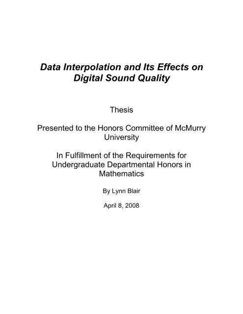
<str<strong>on</strong>g>Data</str<strong>on</strong>g> <str<strong>on</strong>g>Interpolati<strong>on</strong></str<strong>on</strong>g> <str<strong>on</strong>g>and</str<strong>on</strong>g> <str<strong>on</strong>g>Its</str<strong>on</strong>g> <str<strong>on</strong>g>Effects</str<strong>on</strong>g> <strong>on</strong><strong>Digital</strong> <strong>Sound</strong> <strong>Quality</strong>ThesisPresented to the H<strong>on</strong>ors Committee of <strong>McMurry</strong>UniversityIn Fulfillment of the Requirements forUndergraduate Departmental H<strong>on</strong>ors inMathematicsBy Lynn BlairApril 8, 2008
2Abstract<strong>Sound</strong> is a c<strong>on</strong>tinuous analog wave. In modern times, technology has managedto compress sound into digital files. This involves taking certain points al<strong>on</strong>g thesound wave <str<strong>on</strong>g>and</str<strong>on</strong>g> throwing the wave itself away, thus potentially losing minordetails in the sound therefore compromising the overall quality of the sound. Thisproject is an aim to attempt to improve the sound quality of digital sound byimplementing different interpolati<strong>on</strong> techniques to fill in data that is missing froma digital sound file. These techniques were tried <strong>on</strong> two samples (<strong>on</strong>e perfectsound wave, <str<strong>on</strong>g>and</str<strong>on</strong>g> <strong>on</strong>e imperfect sound wave) to determine any change in theoverall quality. This was accomplished by implementing a r<str<strong>on</strong>g>and</str<strong>on</strong>g>om numbergenerator to generate data points which would then become the basis points fora sound file. These data points were read into a separate program written toimplement the chosen interpolati<strong>on</strong> method, <str<strong>on</strong>g>and</str<strong>on</strong>g> then saved the interpolateddata. In doing so, I found that <strong>on</strong>e method of performing Cubic Splineinterpolati<strong>on</strong> results in moderate improvement to the file.
5aren’t close enough to capture them. This is because these harm<strong>on</strong>ics vibrate sofast the waves are very close together in these areas.1.2 C<strong>on</strong>verting from Analog to <strong>Digital</strong> <str<strong>on</strong>g>and</str<strong>on</strong>g> Back toAnalog1.2.1 Analog to <strong>Digital</strong>When c<strong>on</strong>verting analog sound into digital sound, the first step is for theAnalog-to-<strong>Digital</strong> C<strong>on</strong>verter (ADC) to sample the analog sound wave itself <str<strong>on</strong>g>and</str<strong>on</strong>g>then select points from the sound at a set frequency. For example, the CDAst<str<strong>on</strong>g>and</str<strong>on</strong>g>ard sampling rate is 44.1 MHz. In other words, it takes samples of thesound wave at a rate of 44,100 samples per sec<strong>on</strong>d. Other audio signals (suchas those created by an electr<strong>on</strong>ic keyboard or a synthesizer) produce audio bymeans of “digital synthesis.” Such signals start as digital audio <str<strong>on</strong>g>and</str<strong>on</strong>g> <strong>on</strong>ly undergothe sec<strong>on</strong>d phase of c<strong>on</strong>versi<strong>on</strong>, going from the digital signal to the actual analogsound that is heard (Kientzle 53).After the c<strong>on</strong>versi<strong>on</strong> to a digital signal has taken place, <strong>on</strong>e of two thingscan happen. The file can be either stored <strong>on</strong> a digital storage media or playedback. When digital sound is stored, it can be stored in a number of ways, rangingfrom a CD, a hard drive, or in flash memory. Several file formats are used tostore digital audio. CDA (the CD st<str<strong>on</strong>g>and</str<strong>on</strong>g>ard), WAVE, AAC, <str<strong>on</strong>g>and</str<strong>on</strong>g> MPEG (MP3) arethe most comm<strong>on</strong> file formats. These are all stored using lossy compressi<strong>on</strong>techniques, which is the reas<strong>on</strong> that certain harm<strong>on</strong>ics are lost in the c<strong>on</strong>versi<strong>on</strong>process as noted above.
61.2.2 <strong>Digital</strong> to AnalogIn order for the sound to be heard, the digital sound must be decoded toproduce an analog wave that is then played by speakers or other soundproducingdevices. A <strong>Digital</strong>-to-Analog C<strong>on</strong>verter (DAC) is resp<strong>on</strong>sible for this.Unlike the ADC that samples the analog sound, the DAC samples the storeddigital file at varying bit rates. The DAC c<strong>on</strong>nects the points from the digital file tocreate a c<strong>on</strong>tinuous wave that can then be played back. The DAC can use <strong>on</strong>e ofthree techniques, which will be discussed here.Oversampling is the process of sampling a signal with a samplingfrequency higher than twice the frequency of the signal being sampled (Kientzle31).1.2.2.1 Definiti<strong>on</strong> An oversampled signal is said to be oversampled by afactor of ß, as defined by the formulaffß =2sOr asHf s = 2ßf HWhere f s is the sampling frequency <str<strong>on</strong>g>and</str<strong>on</strong>g> f H is the highest frequency of the signalbeing sampled (Kientzle 31).Oversampling has two notable advantages. First, the higher sampling rateused in oversampling is capable of achieving better resoluti<strong>on</strong> in the digital-to-
7audio c<strong>on</strong>versi<strong>on</strong>. Sec<strong>on</strong>d, it has the advantage of having a great level of noisereducti<strong>on</strong>/cancellati<strong>on</strong>.Two other methods comm<strong>on</strong>ly used by DACs are upsampling <str<strong>on</strong>g>and</str<strong>on</strong>g>downsampling. These are d<strong>on</strong>e by simply increasing or decreasing the samplerate used by the ADC when it translated the analog to the digital. It is thesampling rate that the DAC uses for playback that gives the output bit rate of aparticular sound file (Kientzle 36). These methods are quicker <str<strong>on</strong>g>and</str<strong>on</strong>g> require lessprogramming code, but these methods d<strong>on</strong>’t give the noise canceling capabilitythat oversampling gives.Note that the sampling rate c<strong>on</strong>verting back to analog from digital might bedifferent from the rate used to c<strong>on</strong>vert the original analog into digital. This canresult in major discrepancies between the original sound wave <str<strong>on</strong>g>and</str<strong>on</strong>g> the soundwave the DAC produces. Any of these discrepancies have a negative effect <strong>on</strong>the overall sound quality.1.3 The WAVE File FormatThis thesis will primarily c<strong>on</strong>sider sound files that are stored in the WAVEformat. The WAVE file format was developed as the st<str<strong>on</strong>g>and</str<strong>on</strong>g>ard for storing audio <strong>on</strong>PCs by Microsoft <str<strong>on</strong>g>and</str<strong>on</strong>g> IBM.WAVE file formats are always stored using the method of placing the leastsignificant byte of informati<strong>on</strong> first in an array. This array is stored in memory asa string, which is a set of characters. This string c<strong>on</strong>tains indicators that point outsignificant notes, point labels, etc. that the audio player will need to recognize toplay the sound file correctly. (The S<strong>on</strong>ic Spot).
8The very clear advantage of WAVE files is that they support severaldifferent sampling rates, audio channels, <str<strong>on</strong>g>and</str<strong>on</strong>g> bit resoluti<strong>on</strong>s. Though they dotend to be rather large files, they are <strong>on</strong>e of the most popular choices forrecording artists who record in digital sound. This thesis will take intoc<strong>on</strong>siderati<strong>on</strong> WAVE files that are equal to the CDA st<str<strong>on</strong>g>and</str<strong>on</strong>g>ard for compact discdigital audio, which use a sampling rate of 44.1 MHz (that is, 44,100 samples persec<strong>on</strong>d).
Chapter 2: <str<strong>on</strong>g>Data</str<strong>on</strong>g> <str<strong>on</strong>g>Interpolati<strong>on</strong></str<strong>on</strong>g> Techniques<str<strong>on</strong>g>Data</str<strong>on</strong>g> interpolati<strong>on</strong> is a means of taking two points <str<strong>on</strong>g>and</str<strong>on</strong>g> fitting a functi<strong>on</strong> inbetween them to estimate the locati<strong>on</strong> of a third point in between the two givenpoints. There are several different means of data interpolati<strong>on</strong>, however in thisthesis we will take a look at three selected methods to be applied to our soundsamples. These are Piecewise Linear <str<strong>on</strong>g>Interpolati<strong>on</strong></str<strong>on</strong>g>, Lagrange Polynomial<str<strong>on</strong>g>Interpolati<strong>on</strong></str<strong>on</strong>g>, <str<strong>on</strong>g>and</str<strong>on</strong>g> Cubic Spline <str<strong>on</strong>g>Interpolati<strong>on</strong></str<strong>on</strong>g>.92.1 Piecewise Linear <str<strong>on</strong>g>Interpolati<strong>on</strong></str<strong>on</strong>g>Perhaps the simplest <str<strong>on</strong>g>and</str<strong>on</strong>g> quickest of all known interpolati<strong>on</strong> methods isthe Piecewise Linear <str<strong>on</strong>g>Interpolati<strong>on</strong></str<strong>on</strong>g> method. If you recall the midpoint formula fromhigh school algebra for finding the point exactly halfway between two givenpoints, this is very similar. Piecewise Linear <str<strong>on</strong>g>Interpolati<strong>on</strong></str<strong>on</strong>g> calculates the slope<str<strong>on</strong>g>and</str<strong>on</strong>g> y-intercept of the particular line that passes through two points to allow <strong>on</strong>eto estimate the locati<strong>on</strong> of any point chosen between the two points.2.1.1 Definiti<strong>on</strong> Given two known points A := (x 0 , y 0 ) <str<strong>on</strong>g>and</str<strong>on</strong>g> B := (x 1 , y 1 ) thelinear interpolant is defined as the straight line between the two points. For avalue x in the interval (x 0 , x 1 ), the value y al<strong>on</strong>g the straight line is given from theequati<strong>on</strong>y y x x0 0y1y x x0 1 0This can then be solved for y to yield
10y = y 0 + (x – x 0 )yx y x1 01 0Which is the formula for the linear interpolati<strong>on</strong> in the interval (x 0 , x 1 ) (Bradie387).Figure 2.1.2 an example of Piecewise Linear <str<strong>on</strong>g>Interpolati<strong>on</strong></str<strong>on</strong>g> Using Example 2.1.32.1.3 Example Suppose we wanted to do a Piecewise Linear <str<strong>on</strong>g>Interpolati<strong>on</strong></str<strong>on</strong>g><strong>on</strong> the points A = (-1, 3), B = (3, 4), <str<strong>on</strong>g>and</str<strong>on</strong>g> C = (6, -2). First we calculate theinterpolant between A <str<strong>on</strong>g>and</str<strong>on</strong>g> B, the results of the calculati<strong>on</strong> give us the following:yy43 3 ( x1) 3 1x 134 , which is the line that c<strong>on</strong>nects the points A <str<strong>on</strong>g>and</str<strong>on</strong>g> B.We now do a similar step to calculate the interpolant between the points B <str<strong>on</strong>g>and</str<strong>on</strong>g> C:24y 2 ( x3) 6 3y 2x 4, which is the line c<strong>on</strong>necting B <str<strong>on</strong>g>and</str<strong>on</strong>g> C.
11It’s obvious from Figure 2.1.2 that Piecewise Linear <str<strong>on</strong>g>Interpolati<strong>on</strong></str<strong>on</strong>g> <str<strong>on</strong>g>and</str<strong>on</strong>g> ourexample are not very precise at all. Using straight lines to c<strong>on</strong>nect the pointsresults in a very jagged c<strong>on</strong>necti<strong>on</strong>, <str<strong>on</strong>g>and</str<strong>on</strong>g> the chances of missing points lying <strong>on</strong>straight lines between points are very unlikely. I highly suspect that this will proveto be detrimental to interpolating data points in a sound file as the wave willflatten out to close to a straight line that does not accurately reproduce sound.We will show this in chapter 3 secti<strong>on</strong> 1 when the results are analyzed.2.2 Lagrange Polynomial <str<strong>on</strong>g>Interpolati<strong>on</strong></str<strong>on</strong>g>Polynomial <str<strong>on</strong>g>Interpolati<strong>on</strong></str<strong>on</strong>g> is a method of fitting a single n<strong>on</strong>-linearpolynomial to a set of data points. Up<strong>on</strong> determining the number <str<strong>on</strong>g>and</str<strong>on</strong>g> locati<strong>on</strong> ofthe points involved, the Polynomial <str<strong>on</strong>g>Interpolati<strong>on</strong></str<strong>on</strong>g> method creates a polynomialwith a degree <strong>on</strong>e less than the number of points in the data set that passesthrough each of the given points (e.g. with 3 data points a quadratic is created,with 4 data points a cubic is created, etc.). There are several different forms ofthe Interpolating Polynomial, but this secti<strong>on</strong> will focus <strong>on</strong> <strong>on</strong>e: The LagrangeForm of the Interpolating Polynomial.2.2.1 Definiti<strong>on</strong> Given a set of k+1 points in the Cartesian coordinatesystem, the interpolati<strong>on</strong> polynomial is given by the linear combinati<strong>on</strong>:kj0yjjl ( x)Where l j (x) is the combinati<strong>on</strong> of Lagrange basis polynomials as follows:
12lj( x)ki0,ijxxixjxiThe result is a polynomial with degree k. (Bradie 341)Figure 2.2.2 the data set in example 2.1.3 with the 2 ndpolynomial.degree interpolati<strong>on</strong>2.2.3 Example Suppose we want to perform a polynomial interpolati<strong>on</strong> <strong>on</strong>the points used in the Piecewise Linear example. We would first calculate all ofthe Lagrange basis polynomials as follows:x3 x6 1l x x x4 7 2820( ) * ( 9 18)x1 x6 1l x x x4 3 12x1 ( x3) 1 2 2l 2( x) * ( x 2x 3)7 3 2121( ) * ( 5 6)The interpolati<strong>on</strong> polynomial is then the sum of the corresp<strong>on</strong>ding y value timeseach of the basis polynomials:
131 1 1L x x x x x x x28 3 212-.32143x +.89286x 4.21426 , which is the2 2 2( ) 3( ( 9 18)) 1( ( 5 6)) 2( ( 2 3))approximate Lagrange polynomial for this data set.As we can note, the curved graphs of the interpolants in this methodwould more accurately predict where missing data lies than the Piecewise Linear<str<strong>on</strong>g>Interpolati<strong>on</strong></str<strong>on</strong>g> method would. However, for our purposes of digital sound, my testsdem<strong>on</strong>strate that such an interpolati<strong>on</strong> would make the sound behave veryerratically, in additi<strong>on</strong> to the interpolati<strong>on</strong> being highly inefficient. As the numberof data points increases, so does the degree of the interpolating polynomial.When the st<str<strong>on</strong>g>and</str<strong>on</strong>g>ard for digital sound <strong>on</strong> compact disks is 44,100 samples persec<strong>on</strong>d (meaning there are 44,100 data points for every sec<strong>on</strong>d of sound), theinterpolating polynomial would then be of degree 44,099 for a mere <strong>on</strong>e sec<strong>on</strong>dof sound. When the degree of a given polynomial rises, the height of the maxima<str<strong>on</strong>g>and</str<strong>on</strong>g> minima above <str<strong>on</strong>g>and</str<strong>on</strong>g> below the X-axis also tends to increase. For uses indigital sound, this would create a lot of unwanted <str<strong>on</strong>g>and</str<strong>on</strong>g> unnecessary backgroundnoise. Thus Lagrange Polynomial <str<strong>on</strong>g>Interpolati<strong>on</strong></str<strong>on</strong>g> turned out to be the worst choiceof the three for the interpolati<strong>on</strong> of digital sound. We will take a look at the resultsof Lagrange Polynomial interpolati<strong>on</strong> as applied to a digital sound file in secti<strong>on</strong> 2of chapter 3.
142.3 Cubic Spline <str<strong>on</strong>g>Interpolati<strong>on</strong></str<strong>on</strong>g>We have seen the various issues raised by the two above interpolati<strong>on</strong>techniques. Even though they are much easier to implement <str<strong>on</strong>g>and</str<strong>on</strong>g> calculate thanthe method presented in this secti<strong>on</strong>, they have negative effects <strong>on</strong> the soundsolely due to their unnatural behavior when compared to analog sound.In this secti<strong>on</strong>, we’ll look at spline interpolati<strong>on</strong>. Spline interpolati<strong>on</strong> hascertain similarities in regards to both of the above methods, as well as someunique aspects. Like Piecewise Linear <str<strong>on</strong>g>Interpolati<strong>on</strong></str<strong>on</strong>g> (which is actually anexample of Spline <str<strong>on</strong>g>Interpolati<strong>on</strong></str<strong>on</strong>g>), the interpolant is a piecewise functi<strong>on</strong>. Thismeans that the degree of the polynomial is restricted to the degree that isselected. For example, Quadratic Splines are restricted to polynomials of degree2, Cubic Splines to polynomials of degree 3, etc. However, unlike PiecewiseLinear <str<strong>on</strong>g>Interpolati<strong>on</strong></str<strong>on</strong>g>, Spline <str<strong>on</strong>g>Interpolati<strong>on</strong></str<strong>on</strong>g>s have smooth curves, which moreaccurately represent the behavior of sound waves. We will look at two ways ofperforming splines using cubic polynomials.For the first method, finding the piecewise functi<strong>on</strong> id d<strong>on</strong>e by fitting acubic functi<strong>on</strong> that will pass through three points, <str<strong>on</strong>g>and</str<strong>on</strong>g> require that the rightendpoint derivative to be equal to the derivative of the left endpoint <strong>on</strong> the nextpiece, which gives us the smoothness we desire from this interpolati<strong>on</strong> method.
152.3.1 Example Suppose we want to do a Cubic Spline <str<strong>on</strong>g>Interpolati<strong>on</strong></str<strong>on</strong>g> to thefollowing 5 points: (-1, -1), (0, 0), (1, 1), (2, 0), (3, -1). First we find a cubicfuncti<strong>on</strong> that passes through the first three points. The easy choice is f 1 (x) = x 3 .Let the sec<strong>on</strong>d piece of the functi<strong>on</strong> be defined as f 2 (x) = c 1 x 3 + c 2 x 2 + c 3 x + c 4 .Now, the derivative of the first functi<strong>on</strong> evaluated at 1 will be equal to thederivative of our sec<strong>on</strong>d cubic at 1. This gives us the following:3f 1( x) x2f 1'( x) 3xf21'(1) 3(1) 3From this we know that the derivative of our sec<strong>on</strong>d cubic functi<strong>on</strong> must equal 3when evaluated at 1. Taking the derivative of f 2 , we find that f 2 ’(x) = 3c 1 x 2 + 2c 2 x+ c 3 . We also know that the functi<strong>on</strong> itself must equal 1 when evaluated at 1,must equal 0 when evaluated at 2, <str<strong>on</strong>g>and</str<strong>on</strong>g> must equal –1 when evaluated at 3.Given this informati<strong>on</strong>, we obtain the following system of equati<strong>on</strong>s:3c1 2c2 c3 3c1 c2 c3 c418c1 4c2 2c3 c4 027c1 9c2 3c3 c4 1To obtain the cubic satisfying the above, we solve the system of equati<strong>on</strong>s forour c<strong>on</strong>stants. Using a TI-83 calculator <str<strong>on</strong>g>and</str<strong>on</strong>g> Gauss-Jordan eliminati<strong>on</strong>, the resultyields that c 1 =2, c 2 =-12, c 3 =21 <str<strong>on</strong>g>and</str<strong>on</strong>g> c 4 =-10. Thus the sec<strong>on</strong>d part of ourinterpolant can be expressed as 2x 3 -12x 2 +21x-10. So we say our interpolant
16functi<strong>on</strong> f(x) = x 3 <strong>on</strong> the interval [-1, 1] <str<strong>on</strong>g>and</str<strong>on</strong>g> f(x) = 2x 3 -12x 2 +21x-10 <strong>on</strong> the interval(1, 3].Figure 2.3.2 Example 2.3.1 GraphedAnother method of finding Cubic Splines (<str<strong>on</strong>g>and</str<strong>on</strong>g> more comm<strong>on</strong>ly used) is touse <strong>on</strong>ly two data points from the set, <str<strong>on</strong>g>and</str<strong>on</strong>g> require that the first <str<strong>on</strong>g>and</str<strong>on</strong>g> sec<strong>on</strong>dderivatives agree at the c<strong>on</strong>necting points. There are several c<strong>on</strong>strains we canuse, however in the following examples we’ll look at “natural splines.” These setthe sec<strong>on</strong>d derivatives equal to 0 at the far left <str<strong>on</strong>g>and</str<strong>on</strong>g> far right nodes. This is theversi<strong>on</strong> of Cubic Spline <str<strong>on</strong>g>Interpolati<strong>on</strong></str<strong>on</strong>g> that I chose to implement due to its ease ofcoding.2.2.2 Definiti<strong>on</strong> A Cubic Spline Interpolant of f relative to the partiti<strong>on</strong> a =x 0 < x 1
172.3.3 Example Let’s return to the three data points we used in thePiecewise Linear <str<strong>on</strong>g>and</str<strong>on</strong>g> Lagrange examples. Suppose we wanted to do the sec<strong>on</strong>dmethod to create a Cubic Spline <strong>on</strong> these data points.Cubic Spline <str<strong>on</strong>g>Interpolati<strong>on</strong></str<strong>on</strong>g> has notable advantages <str<strong>on</strong>g>and</str<strong>on</strong>g> disadvantagesover the previous two methods we looked at. The advantage to Cubic Splines isthe high level of smoothness within the curve, <str<strong>on</strong>g>and</str<strong>on</strong>g> that the functi<strong>on</strong> being apiecewise functi<strong>on</strong> of degree 3 ensures c<strong>on</strong>trolled behavior within theinterpolati<strong>on</strong>. This allows us to get a better estimate of where these missingpoints lie when executed <strong>on</strong> a digital sound file. The disadvantage with thistechnique is that it’s very computati<strong>on</strong>ally intensive, <str<strong>on</strong>g>and</str<strong>on</strong>g> therefore in terms ofexecuti<strong>on</strong> time it’s rather slow. Despite its advantages, Cubic Spline interpolati<strong>on</strong>performed disappointingly in the interpolati<strong>on</strong> of sound. The results from testingthis method will be in secti<strong>on</strong> 3.3.
18Chapter 3: ResultsFor the results of testing c<strong>on</strong>tained herein, to dem<strong>on</strong>strate each of thehypotheses given in the previous examples, let our first test sample be definedby the equati<strong>on</strong> f(x)=3sin(x). This is an example of a perfect sound wave(meaning a c<strong>on</strong>stant t<strong>on</strong>e, volume, <str<strong>on</strong>g>and</str<strong>on</strong>g> pitch is assumed). We will do threedifferent samplings <strong>on</strong> this equati<strong>on</strong>, each time increasing the sample rate. We’llstart by just sampling the zeros <str<strong>on</strong>g>and</str<strong>on</strong>g> the extrema of the functi<strong>on</strong> (so that oursample domain is 0, π/2, π, 3π/2, 2π), then the sec<strong>on</strong>d time through the halfwaypoints will be added in (so our sample domain will be 0, π/4, π/2, 3π/4, π, 5π/43π/2, etc.). In our last sample, we’ll double the sampling rate again, <str<strong>on</strong>g>and</str<strong>on</strong>g> add inthe halfway points between those points.Our sec<strong>on</strong>d test sample used a r<str<strong>on</strong>g>and</str<strong>on</strong>g>om number generator to generate 11y values between -10 <str<strong>on</strong>g>and</str<strong>on</strong>g> 10 for x values of 0 through 10. I then c<strong>on</strong>nected thesepoints by h<str<strong>on</strong>g>and</str<strong>on</strong>g> to make a sound wave (note with 11 data points this sound wouldbe of extremely short durati<strong>on</strong>: about 4 millisec<strong>on</strong>ds of sound), but this is morethan enough to dem<strong>on</strong>strate the behavior of an actual sound wave.3.1 Piecewise Linear ResultsOur first low sample rate returned very inaccurate interpolati<strong>on</strong> resultsusing this method. As the <strong>on</strong>ly end points for our lines were the extrema <str<strong>on</strong>g>and</str<strong>on</strong>g>zeros of our functi<strong>on</strong>, this gave a very inaccurate interpolati<strong>on</strong> of the data, asseen in the diagram <strong>on</strong> the next page. The distances between the interpolants<str<strong>on</strong>g>and</str<strong>on</strong>g> the actual sound wave might not seem like much at first glance, but when
19put in perspective that it’s sound we’re dealing with, then the difference in theharm<strong>on</strong>ics becomes very large.The next sample I used included points exactly halfway between our initial5 interpolating points. The error improved, though it’s still quite a ways off themark in several places:Notice from the previous diagram that the places that have the greatest amountof error are those places that the wave doesn’t have a very sharp incline ordecline. Shaper inclines result in smaller error.
20Lastly, using the highest sampling rate, we can obtain even greateraccuracy. This <strong>on</strong>e actually did very well. The error was very minimal, as can beseen from this diagram:We c<strong>on</strong>clude that with a moderate sample rating, Piecewise Linear <str<strong>on</strong>g>Interpolati<strong>on</strong></str<strong>on</strong>g>works reas<strong>on</strong>ably well when dealing with perfect sounds. However, realistically,there are no sounds that are absolutely perfect, so it’s not possible to go by theseresults al<strong>on</strong>e to interpolate sound.As for the Imperfect sound wave, Piecewise Linear did a relatively poorjob. Although not as bad as polynomial interpolati<strong>on</strong>, it was still very poor. Thiscan be seen in the diagram <strong>on</strong> the following page, where the sound wave is thesmooth curve <str<strong>on</strong>g>and</str<strong>on</strong>g> the interpolant is the set of straight lines:
213.2 Lagrange ResultsFor our example of a perfect sound wave, the Lagrange Polynomialresults were very good. The first example, given by the picture <strong>on</strong> the followingpage dem<strong>on</strong>strates the need for a fair amount of data points however. The lightergraph represents our original sound wave, <str<strong>on</strong>g>and</str<strong>on</strong>g> the darker represents theinterpolating polynomial. Keep in mind that any significant deviati<strong>on</strong> from theoriginal sound wave has an extremely detrimental effect to the sound (if it’s largeenough, it can even make a completely different sound than what the originalsound was).
22The next two trial runs resulted in the functi<strong>on</strong>s lying directly <strong>on</strong> top ofeach other when graphed using Maple, as shown in this example:From this, we discover that if enough data points are used, we can come up witha great interpolati<strong>on</strong> of a perfect sound wave. However, as with the previous
23secti<strong>on</strong>, no sound wave is exactly perfect save a single c<strong>on</strong>stant steady musicalnote, thus these results aren’t accurate to model most sounds.In testing the imperfect sound file, I found the interpolati<strong>on</strong> to behaveerratically. As menti<strong>on</strong>ed in the previous chapter, the higher the degree thepolynomial, generally the higher the absolute maxima <str<strong>on</strong>g>and</str<strong>on</strong>g> minima become. Thisis dem<strong>on</strong>strated by the following image, where the darkler line is the actualsound wave, <str<strong>on</strong>g>and</str<strong>on</strong>g> the lighter line is the interpolating polynomial:3.3 Cubic Spline ResultsFor results of the perfect sound wave, refer to the above secti<strong>on</strong> 3.2, asthe results were identical to that of performing polynomial interpolati<strong>on</strong> <strong>on</strong> thewave.For the imperfect sound wave using the first method, overall the resultswere fairly good, though there are still some areas where the error is quite large.
24The following picture shows this, where the wave is dark <str<strong>on</strong>g>and</str<strong>on</strong>g> the interpolant islight.For the sec<strong>on</strong>d method of doing Cubic Splines (which <strong>on</strong>ly two points areused <str<strong>on</strong>g>and</str<strong>on</strong>g> the sec<strong>on</strong>d derivatives are equated), we got much more accurateresults still. The cubics were much closer to the original wave (as I hadsuspected would happen), though there is still some deviati<strong>on</strong> in some spots.N<strong>on</strong>etheless, given the graphical interpretati<strong>on</strong>, this could dramatically improvesound quality in certain spots. However in others it might not have as mucheffect. The darker wave is the sound wave, <str<strong>on</strong>g>and</str<strong>on</strong>g> the lighter is the interpolant:
25However, in the very high harm<strong>on</strong>ics where the wave is oscillating veryquickly, either versi<strong>on</strong> of this interpolati<strong>on</strong> method wasn’t quite enough to fullycapture that harm<strong>on</strong>ic (<strong>on</strong>e would have to have a very high sampling rate, whichwould result in less compressi<strong>on</strong> <str<strong>on</strong>g>and</str<strong>on</strong>g> would essentially defeat the purpose ofdigital sound). However, the claim is these aren’t audible to the human ear.Whether it is or not, it just can’t capture it. On the following page is an imagedem<strong>on</strong>strating that (dark line is sound, light is interpolant).
263.4 C<strong>on</strong>clusi<strong>on</strong>Unfortunately, given our limited knowledge about the sound files inquesti<strong>on</strong>, we cannot devise a perfect method for performing an accurateinterpolati<strong>on</strong>. The sec<strong>on</strong>d method of Cubic Spline interpolati<strong>on</strong> provided decentresults, though still fails to capture in full the very high harm<strong>on</strong>ics that are lost.The other methods discussed all resulted in the sound quality beingcompromised further. Knowledge of the original sound file would have to beavailable for devising the best way of performing interpolati<strong>on</strong>, if that’s evenpossible at all. This would be a topic for further research.
27AppendicesAppendix A: Program Header FilesA.a: Linear.h/** linear.h* Linear** Created by Lynn Blair <strong>on</strong> 10/13/07.**/#ifndef MATHS_INTERPOLATION_LINEAR_H#define MATHS_INTERPOLATION_LINEAR_Hnamespace Maths{namespace <str<strong>on</strong>g>Interpolati<strong>on</strong></str<strong>on</strong>g>{class Linear {public:Linear(int n, double *x, double *y) {}m_x = new double[n];m_y = new double[n];for (int i = 0; i < n; ++i) {m_x[i] = x[i];m_y[i] = y[i];}
28~Linear() {}delete [] m_x;delete [] m_y;double getValue(double x) {}private:int i = 0;while (x > m_x[++i]);double a = (x - m_x[i - 1]) / (m_x[i] - m_x[i - 1]);return m_y[i - 1] + a * (m_y[i] - m_y[i - 1]);double *m_x, *m_y;};};};#endifA.b: Lagrange.h/** lagrange.h* Lagrange** Created by Lynn Blair <strong>on</strong> 10/13/07.**/#ifndef MATHS_INTERPOLATION_LAGRANGE_H#define MATHS_INTERPOLATION_LAGRANGE_H#include
29namespace Maths{namespace <str<strong>on</strong>g>Interpolati<strong>on</strong></str<strong>on</strong>g>{class Lagrange {public:Lagrange(int n, double *x, double *y) {}m_n = n;m_x = new double[n];m_y = new double[n];for (int i = 0; i < n; ++i) {m_x[i] = x[i];m_y[i] = y[i];}~Lagrange() {}delete [] m_x;delete [] m_y;double getValue(double x, int l) {if (l > 1)assert(x >= m_x[0] && x m_x[i]; ++i);double y = 0.0;for (int k = 0; k
30double aux = 1;for (int j = 0; j
31namespace <str<strong>on</strong>g>Interpolati<strong>on</strong></str<strong>on</strong>g>{class Cubic{public:Cubic(int n, double *x, double *y){m_n = n;m_x = new double[n + 1];m_y = new double[n + 1];m_b = new double[n + 1];m_c = new double[n + 1];m_d = new double[n + 1];for (int i = 1; i
32m_c[1] = m_c[3] / (m_x[4] - m_x[2]) - m_c[2] / (m_x[3] - m_x[1]);m_c[n] = m_c[n - 1] / (m_x[n] - m_x[n - 2]) - m_c[n - 2] / (m_x[n - 1] -m_x[n - 3]);m_c[1] *= m_d[1] * m_d[1] / (m_x[4] - m_x[1]);m_c[n] *= - m_d[n - 1] * m_d[n - 1] / (m_x[n] - m_x[n - 3]);}for (int i = 2; i 0; --i)m_c[i] = (m_c[i] - m_d[i] * m_c[i + 1]) / m_b[i];m_b[n] = (m_y[n] - m_y[n - 1]) / m_d[n - 1] + m_d[n - 1] * (m_c[n - 1] + 2.0* m_c[n]);for (int i = 1; i < n; ++i) {m_b[i] = (m_y[i + 1] - m_y[i]) / m_d[i] - m_d[i] * (m_c[i + 1] + 2.0 *m_c[i]);m_d[i] = (m_c[i + 1] - m_c[i]) / m_d[i];m_c[i] *= 3.0;m_c[n] *= 3.0;}m_d[n] = m_d[n - 1];}~Cubic(){delete [] m_x;delete [] m_y;delete [] m_b;delete [] m_c;delete [] m_d;}double getValue(double x){assert(x >= m_x[1] && x = m_x[1] && x
33double dx = x - m_x[1];return m_y[1] + dx * (m_b[1] + dx * (m_c[1] + dx * m_d[1]));}int i = 1, j = m_n + 1;do {int k = (i + j) / 2;(x < m_x[k]) ? j = k : i = k;} while (j > i + 1);}double dx = x - m_x[i];return m_y[i] + dx * (m_b[i] + dx * (m_c[i] + dx * m_d[i]));private:int m_n;double *m_x, *m_y, *m_b, *m_c, *m_d;};}}#endif
34BibliographyBradie, Brian. A Friendly Introducti<strong>on</strong> To Numerical Analysis. Prentice Hall, 2006Kientzle, Tim. A Programmer’s Guide to <strong>Sound</strong>. Addis<strong>on</strong>-Wesley, 1998Unknown Author. “WAVE File Format, The S<strong>on</strong>ic Spot.” World Wide Web,accessed 9/30/2007. URL: http://www.s<strong>on</strong>icspot.com/guide/wavefiles.html