"Civil Engineering" section of the FE Supplied-Reference Handbook ...

GEOTECHNICALDefinitionsc = cohesionc c = coefficient of curvature or gradation= (D 30 ) 2 /[(D 60 )(D 10 )], whereD 10 , D 30 , D 60 = particle diameter corresponding to 10%,30%, and 60% finer on grain-size curve.c u = uniformity coefficient = D 60 /D 10e = void ratio = V v /V s , whereV v = volume of voids, andV s = volume of the solids.K = coefficient of permeability = hydraulic conductivity= Q/(iA) (from Darcy's equation), whereQ = discharge ratei = hydraulic gradient = dH/dx,H = hydraulic head,A = cross-sectional area.q u = unconfined compressive strength = 2cw = water content (%) = (W w /W s ) ×100, whereW w = weight of water, andW s = weight of solids.C c = compression index = ∆e/∆log p= (e 1 – e 2 )/(log p 2 – log p 1 ), wheree 1 and e 2 = void ratio, andp 1 and p 2 = pressure.D r = relative density (%)= [(e max – e)/(e max – e min )] ×100= [(1/γ min – 1/γ d ) /(1/γ min – 1/γ max )] × 100, wheree max and e min = maximum and minimum void ratio, andγ max and γ min = maximum and minimum unit dry weight.G s = specific gravity = W s /(V s γ w ), whereγ w = unit weight of water (62.4 lb/ft 3 or 1,000 kg/m 3 ).∆H = settlement = H [C c /(1 + e i )] log [(p i + ∆p)/p i ]= H∆e/(1 + e i ), whereH = thickness of soil layer∆e = change in void ratio, andp = pressure.PI = plasticity index = LL – PL, whereLL = liquid limit, andPL = plasticity limit.S = degree of saturation (%) = (V w /V v ) × 100, whereV w = volume of water,V v = volume of voids.CIVIL ENGINEERINGQKHN fN d= KH(N f /N d ) (for flow nets, Q per unit width),where= coefficient permeability,= total hydraulic head (potential),= number of flow tubes, and= number of potential drops.γ = total unit weight of soil = W/Vγ d = dry unit weight of soil = W s /V= Gγ w /(1 + e) = γ /(1 + w), whereGw = Seγ s = unit weight of solid = W s / V sn = porosity = V v /V = e/(1 + e)τ = general shear strength = c + σtan φ, whereφ = angle of internal friction,σ = normal stress = P/A,P = force, andA = area.K aK pP aH= coefficient of active earth pressure= tan 2 (45 – φ/2)= coefficient of passive earth pressure= tan 2 (45 + φ/2)= active resultant force = 0.5γH 2 K a , where= height of wall.q ult = bearing capacity equation= cN c + γD f N q + 0.5γBN γ , whereN c , N q , and N γ = bearing capacity factorsB = width of strip footing, and= depth of footing below surface.D fFSLαφWC vTt= factor of safety (slope stability)cL + Wcosαtanφ=, whereW sinα= length of slip plane,= slope of slip plane,= angle of friction, and= total weight of soil above slip plane.= coefficient of consolidation = TH 2 /t, where= time factor,= consolidation time.H dr = length of drainage pathn = number of drainage layersC c = compression index for normally consolidated clay= 0.009 (LL – 10)σ′ = effective stress = σ – u, whereσ = normal stress, andu = pore water pressure.93

CIVIL ENGINEERING (continued)UNIFIED SOIL CLASSIFICATION SYSTEM (ASTM D-2487)Coarse-grained soils(More than half of material is larger than No. 200 sieve size)Fine-grained soils(More than half material is smaller than No. 200 sieve)Major DivisionsGravels(More than half of coarse fraction is larger than No.4 sieve size)Sands(More than half of coarse fraction is smallerthan No. 4 sieve size)Clean gravels (Little or nofines)Gravels with fines(Appreciableamount of fines)Clean sands (Little or nofines)Sands withfines(Appreciableamount offines)Silts and clays(Liquid limit lessthan 50)Silts and clays(Liquid limitgreater than 50)Highly organicsoilsGroupSymbolsGM aSM aGWGPGCSWSPSCMLCLOLMHCHOHPtduduTypical NamesWell-graded gravels, gravel-sandmixtures, little or no finesPoorly-graded gravels, gravel-sandmixtures, little or no finesSilty gravels, gravel-sand-silt mixturesClayey gravels, gravel-sand-claymixturesWell-graded sands, gravelly sands, littleor no finesPoorly graded sand, gravelly sands, littleor no finesSilty sands, sand-silt mixturesClayey sands, sand-clay mixturesInorganic silts and very fine sands, rockflour, silty or clayey fine sands, orclayey silts with slight plasticityInorganic clays of low to mediumplasticity, gravelly clays, sandy clays,silty clays, lean claysOrganic silts and organic silty clays oflow plasticityInorganic silts, micaceous ordiatomaceous fine sandy or silty soils,elastic siltsInorganic clays of high plasticity, fatclaysOrganic clays of medium to highplasticity, organic siltsPeat and other highly organic soilsDetermine percentages of sand and gravel from grain-size curve.Depending on percentage of fines (fraction smaller than No. 200 sieve size), coarse-grained soils areclassified as follows:Less than 5 percent: GW, GP, SW, SPMore than 12 percent: GM, GC, SM, SC5 to 12 percent: Borderline cases requiring dual symbols bLaboratory Classification CriteriaD60c u = greater than 4;Dc c =D102( D )1030× D60between 1 and 3Not meeting all gradiation requirements for GWAtterberg limits below "A"line or PI less than 4Atterberg limits above "A"line with PI greater than 7D60c u = greater than 6;Dc c =D10( D )10302× D60Above "A" linewith PI between 4and 7 areborderline casesrequiring use ofdual symbolsbetween 1 and 3Not meeting all gradation requirements for SWAtterberg limits below "A"line or PI less than 4Atterberg limits above "A"line with PI greater than 7Limits plotting inhatched zone withPI between 4 and 7are borderlinecases requiring useof dual symbolsabDivision of GM and SM groups into subdivisions of d and u are for roads and airfields only. Subdivision is based onAtterberg limits; suffix d used when LL is 28 or less and the PI is 6 or less; the suffix u used when LL is greater than 28.Borderline classification, used for soils possessing characteristics of two groups, are designated by combinations of groupsymbols. For example GW-GC, well-graded gravel-sand mixture with clay binder.94

STRUCTURAL ANALYSISInfluence LinesAn influence diagram shows the variation of a function(reaction, shear, bending moment) as a single unit loadmoves across the structure. An influence line is used to (1)determine the position of load where a maximum quantitywill occur and (2) determine the maximum value of thequantity.Deflection of TrussesPrinciple of virtual work as applied to trusses∆∆= Σf Q δL= deflection at point of interestf Q = member force due to virtual unit load applied atthe point of interestδL = change in member length= αL(∆T) for temperature= F p L/AE for external loadαL= coefficient of thermal expansion= member lengthCIVIL ENGINEERING (continued)Fp = member force due to external loadAE= cross-sectional area of member= modulus of elasticity∆T = T–T O ; T = final temperature, and T O = initialtemperatureDeflection of FramesThe principle of virtual work as applied to frames: L mM ∆ = dxO EI m = bending moment as a funtion of x due to virtualunit load applied at the point of interestM = bending moment as a function of x due to externalloadsBEAM FIXED-END MOMENT FORMULASPab2FEM AB =L2Pa2bFEM BA =L2w2 o LFEM AB =12w2 o LFEM BA =12w2 o LFEM AB =30w2 o LFEM BA =20Live Load ReductionThe live load applied to a structure member can be reduced as the loaded area supported by the member is increased. A typicalreduction model (as used in ASCE 7 and in building codes) for a column supporting two or more floors is: 15 Lreduced= L nominal0.25 + ≥ 0.4 Lnominal kLLA T Columns: k LL = 4Beams: k LL = 2where L nominal is the nominal live load (as given in a load standard or building code), A T is the floor tributary area(s) supportedby the member, and k LL is the ratio of the area of influence to the tributary area.95

REINFORCED CONCRETE DESIGN ACI 318-02US Customary unitsDefinitionsa = depth of equivalent rectangular stress block, inA g = gross area of column, in 2A s = area of tension reinforcement, in 2A s ' = area of compression reinforcement, in 2A st = total area of longitudinal reinforcement, in 2A v = area of shear reinforcment within a distance s, inb = width of compression face of member, inb e = effective compression flange width, inb w = web width, inβ 1 = ratio of depth of rectangular stress block, a, to depthto neutral axis, cf c= ' − 4,000 0.85 ≥ 0.85 – 0.05 ≥ 0.65 1,000 c = distance from extreme compression fiber to neutralaxis, ind = distance from extreme compression fiber to centroidof nonprestressed tension reinforcement, ind t = distance from extreme tension fiber to extremetension steel, in1.5E c = modulus of elasticity = 33 w c f c ' , psiε t = net tensile strain in extreme tension steel at nominalstrengthf c ' = compressive strength of concrete, psif y = yield strength of steel reinforcement, psih f = T-beam flange thickness, inM c = factored column moment, including slendernesseffect, in-lbM n = nominal moment strength at section, in-lbφM n = design moment strength at section, in-lbM u = factored moment at section, in-lbP n = nominal axial load strength at given eccentricity, lbφP n = design axial load strength at giveneccentricity, lbP u = factored axial force at section, lbρ g = ratio of total reinforcement area to cross-sectionalarea of column = A st /A gs = spacing of shear ties measured along longitudinalaxis of member, inV c = nominal shear strength provided by concrete, lbV n = nominal shear strength at section, lbφV n = design shear strength at section, lbV s = nominal shear strength provided by reinforcement,lbV u = factored shear force at section, lbCIVIL ENGINEERING (continued)ASTM STANDARD REINFORCING BARSBAR SIZE DIAMETER, IN AREA, IN 2 WEIGHT, LB/FT#3 0.375 0.11 0.376#4 0.500 0.20 0.668#5 0.625 0.31 1.043#6 0.750 0.44 1.502#7 0.875 0.60 2.044#8 1.000 0.79 2.670#9 1.128 1.00 3.400#10 1.270 1.27 4.303#11 1.410 1.56 5.313#14 1.693 2.25 7.650#18 2.257 4.00 13.60LOAD FACTORS FOR REQUIRED STRENGTHU = 1.4 DU = 1.2 D + 1.6 LSELECTED ACI MOMENT COEFFICIENTSApproximate moments in continuous beams of three ormore spans, provided:1. Span lengths approximately equal (length oflonger adjacent span within 20% of shorter)2. Uniformly distributed load3. Live load not more than three times dead load2M u = coefficient * w u * L nw u = factored load per unit beam lengthL n = clear span for positive moment; averageadjacent clear spans for negative momentColumnSpandrelbeam− 161− 241+ 141L n+ 1411Unrestrained + 11end− 101− 101− 101− 111− 111− 111+ 161+ 161+ 161− 111− 111− 11196End spanInterior span

CIVIL ENGINEERING (continued)BEAMS − FLEXURE: φM N ≥ M U (CONTINUED)BEAMS − SHEAR:φV N ≥ V uDoubly-reinforced beams (continued)Compression steel does not yield (continued) c − d'2. f s '=87,000 c 0.85f 3. A s,max =c ' β1 b 3d t − A s ' f s 'f y 7 f y ( Asf y − As' fs')4. a =0.85 fc' bAsf y aM n = f s ' − As' d − + As' ( d − d') fs'2 T-beams − tension reinforcement in stemEffective flange width:Beam width used in shear equations:b w =b (rectangular beams )b w (T−beams)Nominal shear strength:V n = V c + V sV c = 2 b w d f c 'A f dV s =v ys[may not exceed 8 b w d f c' ]Required and maximum-permitted stirrup spacing, sφVcVu≤ : No stirrups required2φVcVu> : Use the following table ( A v given ):21/4 • span lengthb e = b w + 16 • h fsmallest beam centerline spacingDesign moment strenth:Asf ya =0.85 f c ' beIf a ≤ h f :0.85f c ' β1 be 3 d tA s,max =f 7yRequiredspacingφV2c< VuSmaller of:Avf ys =50bw≤ φVAvf ys =0.75bwf c 'cV u > φV cV s = V u − φV c :φ Avfs =VsydM n = 0.85 f c ' a b e (d- 2a )If a > h f :A s,max =.85 fc' β bf 3d 70 1 e tyM n = 0.85 f c ' [h f (b e − b w ) (d − 0.85f c '(be−bw) h + fh f2)y+ a b w (d − 2a )]fMaximumpermittedspacingSmaller of:s = 2dORs =24"V s ≤ 4 b w dSmaller of:s = 2dORs =24"V s > 4 b w dSmaller of:ds = 4f c 'f c 's =12"98

CIVIL ENGINEERING (continued)SHORT COLUMNS:Reinforcement limits:Astρg=Ag0.01 ≤ ρ g ≤ 0.08Definition of a short column:KL 12M1≤ 34 −rM 2where: KL = L col clear height of column[assume K = 1.0]r = 0.288h rectangular column, h is side lengthperpendicular to buckling axis ( i.e.,side length in the plane of buckling )r = 0.25h circular column, h = diameterM 1 = smaller end momentM 2 = larger end momentConcentrically-loaded short columns: φP n ≥ P uM 1 = M 2 = 0KL≤ 22rDesign column strength, spiral columns: φ = 0.70φP n = 0.85φ [ 0.85 f c ' ( A g − A st ) + A st f y ]Design column strength, tied columns: φ = 0.65φP n = 0.80φ [ 0.85 f c ' ( A g − A st ) + A st f y ]Short columns with end moments:M u = M 2 or M u = P u eUse Load-moment strength interaction diagram to:1. Obtain φP n at applied moment M u2. Obtain φP n at eccentricity e3. Select A s for P u , M uMM12LONG COLUMNS − Braced (non-sway) framesDefinition of a long column:KL 12M1> 34 −rM 2Critical load:2π EIP c =2( KL )π2E I=2( Lcol)where: EI = 0.25 E c I gConcentrically-loaded long columns:e min = (0.6 + 0.03h) minimum eccentricityM 1 = M 2 = P u e min (positive curvature)KL> 22rMcM 2=Pu1 −0.75PcUse Load-moment strength interaction diagramto design/analyze column for P u , M uLong columns with end moments:M 1 = smaller end momentM 2 = larger end momentM 1 positive if M1 , M 2 produce single curvatureMC m2=0.6+0.4 MM21≥0.4CmM 2M c =≥ M 2Pu1 −0.75PcUse Load-moment strength interaction diagramto design/analyze column for P u , M u99

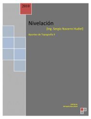
CIVIL ENGINEERING (continued)GRAPH A.11Column strength interaction diagram for rectangular section with bars on end faces and γ = 0.80 (for instructional use only).Design of Concrete Structures, 13th Edition (2004), Nilson, Darwin, DolanMcGraw-Hill ISBN 0-07-248305-9 GRAPH A.11, Page 762Used by permission100

STEEL STRUCTURESReferences: AISC LRFD Manual, 3rd EditionAISC ASD Manual, 9th EditionLOAD COMBINATIONS (LRFD)Floor systems: 1.4D1.2D + 1.6LRoof systems: 1.2D + 1.6(L r or S or R) + 0.8W1.2D + 0.5(L r or S or R) + 1.3W0.9D ± 1.3Wwhere: D = dead load due to the weight of the structure and permanent featuresL = live load due to occupancy and moveable equipmentL r = roof live loadS = snow loadR = load due to initial rainwater (excluding ponding) or iceW = wind loadTENSION MEMBERS: flat plates, angles (bolted or welded)Gross area: A g = b g t (use tabulated value for angles)Net area: A n = (b g − ΣD h +where:b g = gross widtht = thickness2s) t across critical chain of holes4gs = longitudinal center-to-center spacing (pitch) of two consecutive holesg = transverse center-to-center spacing (gage) between fastener gage linesD h = bolt-hole diameterCIVIL ENGINEERING (continued)A e = UA nEffective area (bolted members):U = 1.0 (flat bars)U = 0.85 (angles with ≥ 3 bolts in line)U = 0.75 (angles with 2 bolts in line)LRFDEffective area (welded members):U = 1.0 (flat bars, L ≥ 2w)A e = UA g U = 0.87 (flat bars, 2w > L ≥ 1.5w)U = 0.75 (flat bars, 1.5w > L ≥ w)U = 0.85 (angles)Yielding: φT n = φ y A g F y = 0.9 A g F yFracture: φT n = φ f A e F u = 0.75 A e F uBlock shear rupture (bolted tension members):A gt =gross tension areaA gv =gross shear areaA nt =net tension areaA nv =net shear areaWhen F u A nt ≥ 0.6 F u A nv :φR n =smallerWhen F u A nt < 0.6 F u A nv :φR n =smaller0.75 [0.6 F y A gv + F u A nt ]0.75 [0.6 F u A nv + F u A nt ]0.75 [0.6 F u A nv + F y A gt ]0.75 [0.6 F u A nv + F u A nt ]0ASDYielding: T a = A g F t = A g (0.6 F y )Fracture: T a = A e F t = A e (0.5 F u )Block shear rupture (bolted tension members):T a = (0.30 F u ) A nv + (0.5 F u ) A ntA nt = net tension areaA nv = net shear area102

CIVIL ENGINEERING (continued)BEAMS: homogeneous beams, flexure about x-axisFlexure – local buckling:No local buckling if section is compact:b f 652tf≤ andFyh 640≤t w F ywhere:b f hFor rolled sections, use tabulated values of and2tf t wFor built-up sections, h is clear distance between flangesFor F y ≤ 50 ksi, all rolled shapes except W6 × 19 are compact.Flexure – lateral-torsional buckling: L b = unbraced lengthLp300ry=FLyryX 1L r =+Fwhere: F L = F y – 10 ksiXX1φ = 0.90=φM p = φ F y Z xφM r = φ F L S xCbL b ≤ L p :=2.5 ML p < L b ≤ L r :LRFD–compact rolled shapes21 + 1 X 2 FLπSxCEGJA2S2w x 2 = 4 I y GJ max12.5 M+ 3 MφM n = φM pAmax+ 4 MB+ 3 M L φM n = b − LpC b φMp − ( φMp − φMr) Lr− LpL b > L r :Z x Table= C b [φM p − BF (L b − L p )] ≤ φM pCSee Z x Table for BFZ x TableW-ShapesDimensionsand PropertiesTableLcyASD–compact rolled shapes76bf 20,000= oruse smallerF ( d / A ) FfC b = 1.75 + 1.05(M 1 /M 2 ) + 0.3(M 1 /M 2 ) 2 ≤ 2.3M 1 is smaller end momentM 1 /M 2 is positive for reverse curvatureM a = S F bL b ≤ L c : F b = 0.66 F yL b > L c :For:For:F b22 Fy ( Lb/ rT)= − ≤ 0.6 F y31530 , , 000Cb F b170,000Cb =≤ 0.6 F2y( L / r )F b =bbT12,000CL d / AyfbTy≤ 0.6 F y102, 000CbLb510,000Cb< ≤:F r FUse larger of (F1-6) and (F1-8)Lb510,000Cb> :r FTyUse larger of (F1-7) and (F1-8)y(F1-6)(F1-7)(F1-8)φCbS x X12 XφM n =1 +L /r 2See Beam Design Moments curveby212( L /r ) 2bXy≤ φM pSee Allowable Moments in Beams curve103

Shear – unstiffened beamsLRFD – E = 29,000 ksiφ = 0.90 A w = d t wForASDh 380≤ : F v = 0.40 F yt w F yCIVIL ENGINEERING (continued)h 417≤ φV n = φ (0.6 F y ) A wt w F y417Fy 380w F : F v = Fy( Cv)y2.89where for unstiffened beams:k v = 5.34≤ 0.4 F yφV n = φ (0.6 F y ) A w417( h/t )w F yC v =190 kv439=h/t F ( h/t ) Fwywy523Fh 1.5:φF cr = φ0.8772λ c See Table 3-50: Design Stress for CompressionF yMembers (F y = 50 ksi, φ = 0.85)ASDColumn slenderness parameter:C c =22πF yEAllowable stress for axially loaded columns (doublysymmetric section, no local buckling):WhenWhen KL r F a = KL r max≤ C c2( KL/r)1−2 Fy2Cc5 3( KL/r)(KL / r)+ −3 8C8Cmaxc> C c : F a =3c3212πE23( KL / r )See Table C-50: Allowable Stress for CompressionMembers (F y = 50 ksi)2104

Bearing strengthLRFDDesign strength (kips/bolt/inch thickness):φr n = φ 1.2 L c F u ≤ φ 2.4 d b F uφ = 0.75L c = clear distance between edge of holeand edge of adjacent hole, or edge ofmember, in direction of forceL c = s – D hL c = L e –D h2Design bearing strength (kips/bolt/inchthickness) for various bolt spacings, s,and end distances, L e :Bearingstrengthφr n (k/bolt/inBolt size3/4" 7/8" 1"s = 2 2 / 3 d b ( minimum permitted )F u = 58 ksiF u = 65 ksiF u = 58 ksiF u = 65 ksiF u = 58 ksiF u = 65 ksiF u = 58 ksiF u = 65 ksi62.069.5s = 3"72.981.778.3 91.387.7 102L e = 1 1/4"44.049.4L e = 2"78.387.740.845.779.989.683.793.810111337.542.076.785.9CIVIL ENGINEERING (continued)ASDDesign strength (kips/bolt/inch thickness):When s ≥ 3 d b and L e ≥ 1.5 d br b = 1.2 F u d bWhen L e < 1.5 d b : r b =When s < 3 d b :r b = d b s − F 2 2uL e F u2≤ 1.2 F u d bDesign bearing strength (kips/bolt/inchthickness) for various bolt spacings, s,and end distances, L e :Bearingstrengthr b (k/bolt/in)F u = 58 ksiF u = 65 ksiBolt size3/4" 7/8" 1"s ≥ 3 d b and L e ≥ 1.5 d b52.258.560.968.3s = 2 2/3 d b (minimum permitted)F u = 58 ksiF u = 65 ksiF u = 58 ksiF u = 65 ksi47.152.855.061.6L e = 1 1/4"36.3 [all bolt sizes]40.6 [all bolt sizes]69.678.062.870.4The bearing resistance of the connection shall be taken asthe sum of the bearing resistances of the individual bolts.106

CIVIL ENGINEERING (continued)Area Depth Web Flange Compact X 1 X 2 r T d/A f Axis X-X Axis Y-YShape A d t w b f t f section x 10 6 ** ** I S r Z I rin. 2 in. in. in. in. b f /2t f h/t w ksi 1/ksi in. 1/in. in. 4 in. 3 in. in. 3 in. 4 in.W24 × 103 30.3 24.5 0.55 9.00 0.98 4.59 39.2 2390 5310 2.33 2.78 3000 245 9.96 280 119 1.99W24 × 94 27.7 24.3 0.52 9.07 0.88 5.18 41.9 2180 7800 2.33 3.06 2700 222 9.87 254 109 1.98W24 × 84 24.7 24.1 0.47 9.02 0.77 5.86 45.9 1950 12200 2.31 3.47 2370 196 9.79 224 94.4 1.95W24 × 76 22.4 23.9 0.44 8.99 0.68 6.61 49.0 1760 18600 2.29 3.91 2100 176 9.69 200 82.5 1.92W24 × 68 20.1 23.7 0.42 8.97 0.59 7.66 52.0 1590 29000 2.26 4.52 1830 154 9.55 177 70.4 1.87W24 × 62 18.3 23.7 0.43 7.04 0.59 5.97 49.7 1730 23800 1.71 5.72 1560 132 9.24 154 34.5 1.37W24 × 55 16.3 23.6 0.40 7.01 0.51 6.94 54.1 1570 36500 1.68 6.66 1360 115 9.13 135 29.1 1.34W21 × 93 27.3 21.6 0.58 8.42 0.93 4.53 32.3 2680 3460 2.17 2.76 2070 192 8.70 221 92.9 1.84W21 × 83 24.3 21.4 0.52 8.36 0.84 5.00 36.4 2400 5250 2.15 3.07 1830 171 8.67 196 81.4 1.83W21 × 73 21.5 21.2 0.46 8.30 0.74 5.60 41.2 2140 8380 2.13 3.46 1600 151 8.64 172 70.6 1.81W21 × 68 20.0 21.1 0.43 8.27 0.69 6.04 43.6 2000 10900 2.12 3.73 1480 140 8.60 160 64.7 1.80W21 × 62 18.3 21.0 0.40 8.24 0.62 6.70 46.9 1820 15900 2.10 4.14 1330 127 8.54 144 57.5 1.77* W21 × 55 16.2 20.8 0.38 8.22 0.52 7.87 50.0 1630 25800 --- --- 1140 110 8.40 126 48.4 1.73* W21 × 48 14.1 20.6 0.35 8.14 0.43 9.47 53.6 1450 43600 --- --- 959 93.0 8.24 107 38.7 1.66W21 × 57 16.7 21.1 0.41 6.56 0.65 5.04 46.3 1960 13100 1.64 4.94 1170 111 8.36 129 30.6 1.35W21 × 50 14.7 20.8 0.38 6.53 0.54 6.10 49.4 1730 22600 1.60 5.96 984 94.5 8.18 110 24.9 1.30W21 × 44 13.0 20.7 0.35 6.50 0.45 7.22 53.6 1550 36600 1.57 7.06 843 81.6 8.06 95.4 20.7 1.26* LRFD Manual only ** AISC ASD Manual, 9th Edition107

CIVIL ENGINEERING (continued)Table 1-1: W-Shapes Dimensions and Properties (continued)Area Depth Web Flange Compact X 1 X 2 r Td/A f Axis X-X Axis Y-YShape A d t w b f t fsection x 10 6 ** ** I S r Z I rin. 2 in. in. in. in. b f /2t f h/t w ksi 1/ksi in. 1/in. in. 4 in. 3 in. in. 3 in. 4 in.W18 × 86 25.3 18.4 0.48 11.1 0.77 7.20 33.4 2460 4060 2.97 2.15 1530 166 7.77 186 175 2.63W18 × 76 22.3 18.2 0.43 11.0 0.68 8.11 37.8 2180 6520 2.95 2.43 1330 146 7.73 163 152 2.61W18 × 71 20.8 18.5 0.50 7.64 0.81 4.71 32.4 2690 3290 1.98 2.99 1170 127 7.50 146 60.3 1.70W18 × 65 19.1 18.4 0.45 7.59 0.75 5.06 35.7 2470 4540 1.97 3.22 1070 117 7.49 133 54.8 1.69W18 × 60 17.6 18.2 0.42 7.56 0.70 5.44 38.7 2290 6080 1.96 3.47 984 108 7.47 123 50.1 1.68W18 × 55 16.2 18.1 0.39 7.53 0.63 5.98 41.1 2110 8540 1.95 3.82 890 98.3 7.41 112 44.9 1.67W18 × 50 14.7 18.0 0.36 7.50 0.57 6.57 45.2 1920 12400 1.94 4.21 800 88.9 7.38 101 40.1 1.65W18 × 46 13.5 18.1 0.36 6.06 0.61 5.01 44.6 2060 10100 1.54 4.93 712 78.8 7.25 90.7 22.5 1.29W18 × 40 11.8 17.9 0.32 6.02 0.53 5.73 50.9 1810 17200 1.52 5.67 612 68.4 7.21 78.4 19.1 1.27W18 × 35 10.3 17.7 0.30 6.00 0.43 7.06 53.5 1590 30800 1.49 6.94 510 57.6 7.04 66.5 15.3 1.22W16 × 89 26.4 16.8 0.53 10.4 0.88 5.92 25.9 3160 1460 2.79 1.85 1310 157 7.05 177 163 2.48W16 × 77 22.9 16.5 0.46 10.3 0.76 6.77 29.9 2770 2460 2.77 2.11 1120 136 7.00 152 138 2.46W16 × 67 20.0 16.3 0.40 10.2 0.67 7.70 34.4 2440 4040 2.75 2.40 970 119 6.97 132 119 2.44W16 × 57 16.8 16.4 0.43 7.12 0.72 4.98 33.0 2650 3400 1.86 3.23 758 92.2 6.72 105 43.1 1.60W16 × 50 14.7 16.3 0.38 7.07 0.63 5.61 37.4 2340 5530 1.84 3.65 659 81.0 6.68 92.0 37.2 1.59W16 × 45 13.3 16.1 0.35 7.04 0.57 6.23 41.1 2120 8280 1.83 4.06 586 72.7 6.65 82.3 32.8 1.57W16 × 40 11.8 16.0 0.31 7.00 0.51 6.93 46.5 1890 12700 1.82 4.53 518 64.7 6.63 73.0 28.9 1.57W16 × 36 10.6 15.9 0.30 6.99 0.43 8.12 48.1 1700 20400 1.79 5.28 448 56.5 6.51 64.0 24.5 1.52W16 × 31 9.1 15.9 0.28 5.53 0.44 6.28 51.6 1740 19900 1.39 6.53 375 47.2 6.41 54.0 12.4 1.17W16 × 26 7.7 15.7 0.25 5.50 0.35 7.97 56.8 1480 40300 1.36 8.27 301 38.4 6.26 44.2 9.59 1.12W14 × 120 35.3 14.5 0.59 14.7 0.94 7.80 19.3 3830 601 4.04 1.05 1380 190 6.24 212 495 3.74W14 × 109 32.0 14.3 0.53 14.6 0.86 8.49 21.7 3490 853 4.02 1.14 1240 173 6.22 192 447 3.73W14 × 99 29.1 14.2 0.49 14.6 0.78 9.34 23.5 3190 1220 4.00 1.25 1110 157 6.17 173 402 3.71W14 × 90 26.5 14.0 0.44 14.5 0.71 10.2 25.9 2900 1750 3.99 1.36 999 143 6.14 157 362 3.70W14 × 82 24.0 14.3 0.51 10.1 0.86 5.92 22.4 3590 849 2.74 1.65 881 123 6.05 139 148 2.48W14 × 74 21.8 14.2 0.45 10.1 0.79 6.41 25.4 3280 1200 2.72 1.79 795 112 6.04 126 134 2.48W14 × 68 20.0 14.0 0.42 10.0 0.72 6.97 27.5 3020 1660 2.71 1.94 722 103 6.01 115 121 2.46W14 × 61 17.9 13.9 0.38 9.99 0.65 7.75 30.4 2720 2470 2.70 2.15 640 92.1 5.98 102 107 2.45W14 × 53 15.6 13.9 0.37 8.06 0.66 6.11 30.9 2830 2250 2.15 2.62 541 77.8 5.89 87.1 57.7 1.92W14 × 48 14.1 13.8 0.34 8.03 0.60 6.75 33.6 2580 3250 2.13 2.89 484 70.2 5.85 78.4 51.4 1.91W12 × 106 31.2 12.9 0.61 12.2 0.99 6.17 15.9 4660 285 3.36 1.07 933 145 5.47 164 301 3.11W12 × 96 28.2 12.7 0.55 12.2 0.90 6.76 17.7 4250 407 3.34 1.16 833 131 5.44 147 270 3.09W12 × 87 25.6 12.5 0.52 12.1 0.81 7.48 18.9 3880 586 3.32 1.28 740 118 5.38 132 241 3.07W12 × 79 23.2 12.4 0.47 12.1 0.74 8.22 20.7 3530 839 3.31 1.39 662 107 5.34 119 216 3.05W12 × 72 21.1 12.3 0.43 12.0 0.67 8.99 22.6 3230 1180 3.29 1.52 597 97.4 5.31 108 195 3.04W12 × 65 19.1 12.1 0.39 12.0 0.61 9.92 24.9 2940 1720 3.28 1.67 533 87.9 5.28 96.8 174 3.02W12 × 58 17.0 12.2 0.36 10.0 0.64 7.82 27.0 3070 1470 2.72 1.90 475 78.0 5.28 86.4 107 2.51W12 × 53 15.6 12.1 0.35 9.99 0.58 8.69 28.1 2820 2100 2.71 2.10 425 70.6 5.23 77.9 95.8 2.48W12 × 50 14.6 12.2 0.37 8.08 0.64 6.31 26.8 3120 1500 2.17 2.36 391 64.2 5.18 71.9 56.3 1.96W12 × 45 13.1 12.1 0.34 8.05 0.58 7.00 29.6 2820 2210 2.15 2.61 348 57.7 5.15 64.2 50.0 1.95W12 × 40 11.7 11.9 0.30 8.01 0.52 7.77 33.6 2530 3360 2.14 2.90 307 51.5 5.13 57.0 44.1 1.94** AISC ASD Manual, 9th Edition108

F y = 50 ksiφ b = 0.9φ v = 0.9Table 5-3W-ShapesSelection by Z xCIVIL ENGINEERING (continued)Z xShapeX-X AXISZ x I x φ b M p φ b M r L p L r BF φ v V nin. 3 in. 4 kip-ft kip-ft ft ft kips kipsW 24 × 55 135 1360 506 345 4.73 12.9 19.8 252W 18 × 65 133 1070 499 351 5.97 17.1 13.3 224W 12 × 87 132 740 495 354 10.8 38.4 5.13 174W 16 × 67 131 963 491 354 8.65 23.8 9.04 174W 10 × 100 130 623 488 336 9.36 50.8 3.66 204W 21 × 57 129 1170 484 333 4.77 13.2 17.8 231W 21 × 55 126 1140 473 330 6.11 16.1 14.3 211W 14 × 74 126 796 473 336 8.76 27.9 7.12 173W 18 × 60 123 984 461 324 5.93 16.6 12.9 204W 12 × 79 119 662 446 321 10.8 35.7 5.03 157W 14 × 68 115 722 431 309 8.69 26.4 6.91 157W 10 × 88 113 534 424 296 9.29 45.1 3.58 176W 18 × 55 112 890 420 295 5.90 16.1 12.2 191W 21 × 50 111 989 416 285 4.59 12.5 16.5 213W 12 × 72 108 597 405 292 10.7 33.6 4.93 143W 21 × 48 107 959 401 279 6.09 15.4 13.2 195W 16 × 57 105 758 394 277 5.65 16.6 10.7 190W 14 × 61 102 640 383 277 8.65 25.0 6.50 141W 18 × 50 101 800 379 267 5.83 15.6 11.5 173W 10 × 77 97.6 455 366 258 9.18 39.9 3.53 152W 12 × 65 96.8 533 363 264 11.9 31.7 5.01 127W 21 × 44 95.8 847 359 246 4.45 12.0 15.0 196W 16 × 50 92.0 659 345 243 5.62 15.7 10.1 167W 18 × 46 90.7 712 340 236 4.56 12.6 12.9 176W 14 × 53 87.1 541 327 233 6.78 20.1 7.01 139W 12 × 58 86.4 475 324 234 8.87 27.0 4.97 119W 10 × 68 85.3 394 320 227 9.15 36.0 3.45 132W 16 × 45 82.3 586 309 218 5.55 15.1 9.45 150W 18 × 40 78.4 612 294 205 4.49 12.0 11.7 152W 14 × 48 78.4 485 294 211 6.75 19.2 6.70 127W 12 × 53 77.9 425 292 212 8.76 25.6 4.78 113W 10 × 60 74.6 341 280 200 9.08 32.6 3.39 116W 16 × 40 73.0 518 274 194 5.55 14.7 8.71 132W 12 × 50 71.9 391 270 193 6.92 21.5 5.30 122W 14 × 43 69.6 428 261 188 6.68 18.2 6.31 113W 10 × 54 66.6 303 250 180 9.04 30.2 3.30 101W 18 × 35 66.5 510 249 173 4.31 11.5 10.7 143W 12 × 45 64.2 348 241 173 6.89 20.3 5.06 109W 16 × 36 64.0 448 240 170 5.37 14.1 8.11 127W 14 × 38 61.1 383 229 163 5.47 14.9 7.05 118W 10 × 49 60.4 272 227 164 8.97 28.3 3.24 91.6W 12 × 40 57.0 307 214 155 68.5 19.2 4.79 94.8W 10 × 45 54.9 248 206 147 7.10 24.1 3.44 95.4W 14 × 34 54.2 337 203 145 5.40 14.3 6.58 108109

110CIVIL ENGINEERING (continued)

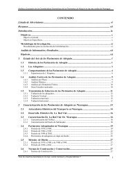
Table C – C.2.1. K VALUES FOR COLUMNSCIVIL ENGINEERING (continued)Theoretical K value 0.5 0.7 1.0 1.0 2.0 2.0Recommended designvalue when ideal conditionsare approximated0.65 0.80 1.2 1.0 2.10 2.0Figure C – C.2.2.ALIGNMENT CHART FOR EFFECTIVE LENGTH OF COLUMNS IN CONTINUOUS FRAMESThe subscripts A and B refer to the joints at the two ends of the column section beingconsidered. G is defined asΣG =Σ( I /L )c c( I /L )ggin which Σ indicates a summation of all members rigidly connected to that joint and lyingon the plane in which buckling of the column is being considered. I c is the moment ofinertia and L c the unsupported length of a column section, and I g is the moment of inertiaand L g the unsupported length of a girder or other restraining member. I c and I g aretaken about axes perpendicular to the plane of buckling being considered.For column ends supported by but not rigidly connected to a footing or foundation, G istheoretically infinity, but, unless actually designed as a true friction-free pin, may betaken as "10" for practical designs. If the column end is rigidly attached to a properlydesigned footing, G may be taken as 1.0. Smaller values may be used if justified byanalysis.111

112CIVIL ENGINEERING (continued)

CIVIL ENGINEERING (continued)F y = 50 ksiALLOWABLE STRESS DESIGN SELECTION TABLEFor shapes used as beamsS xF y = 36 ksiS xFt Ft Kip-ft In. 3 Ft Ft Kip-ftL c L u M R SHAPE L c L u M R5.0 6.3 314 114 W 24 X 55 7.0 7.5 2269.0 18.6 308 112 W 14 x 74 10.6 25.9 2225.9 6.7 305 111 W 21 x 57 6.9 9.4 2206.8 9.6 297 108 W 18 x 60 8.0 13.3 21410.8 24.0 294 107 W 12 x 79 12.8 33.3 2129.0 17.2 283 103 W 14 x 68 10.6 23.9 2046.7 8.7 270 98.3 W 18 X 55 7.9 12.1 19510.8 21.9 268 97.4 W 12 x 72 12.7 30.5 1935.6 6.0 260 94.5 W 21 X 50 6.9 7.8 1876.4 10.3 254 92.2 W 16 x 57 7.5 14.3 1839.0 15.5 254 92.2 W 14 x 61 10.6 21.5 1836.7 7.9 244 88.9 W 18 X 50 7.9 11.0 17610.7 20.0 238 87.9 W 12 x 65 12.7 27.7 1744.7 5.9 224 81.6 W 21 X 44 6.6 7.0 1626.3 9.1 223 81.0 W 16 x 50 7.5 12.7 1605.4 6.8 217 78.8 W 18 x 46 6.4 9.4 1569.0 17.5 215 78.0 W 12 x 58 10.6 24.4 1547.2 12.7 214 77.8 W 14 x 53 8.5 17.7 1546.3 8.2 200 72.7 W 16 x 45 7.4 11.4 1449.0 15.9 194 70.6 W 12 x 53 10.6 22.0 1407.2 11.5 193 70.3 W 14 x 48 8.5 16.0 1395.4 5.9 188 68.4 W 18 X 40 6.3 8.2 1359.0 22.4 183 66.7 W 10 x 60 10.6 31.1 1326.3 7.4 178 64.7 W 16 X 40 7.4 10.2 1287.2 14.1 178 64.7 W 12 x 50 8.5 19.6 1287.2 10.4 172 62.7 W 14 x 43 8.4 14.4 1249.0 20.3 165 60.0 W 10 x 54 10.6 28.2 1197.2 12.8 160 58.1 W 12 x 45 8.5 17.7 1154.8 5.6 158 57.6 W 18 X 35 6.3 6.7 1146.3 6.7 115 56.5 W 16 x 36 7.4 8.8 1126.1 8.3 150 54.6 W 14 x 38 7.1 11.5 1089.0 18.7 150 54.6 W 10 x 49 10.6 26.0 1087.2 11.5 143 51.9 W 12 x 40 8.4 16.0 1037.2 16.4 135 49.1 W 10 x 45 8.5 22.8 976.0 7.3 134 48.6 W 14 X 34 7.1 10.2 964.9 5.2 130 47.2 W 16 X 31 5.8 7.1 935.9 9.1 125 45.6 W 12 x 35 6.9 12.6 907.2 14.2 116 42.1 W 10 x 39 8.4 19.8 836.0 6.5 116 42.0 W 14 X 30 7.1 8.7 835.8 7.8 106 38.6 W 12 X 30 6.9 10.8 764.0 5.1 106 38.4 W 16 x 26 5.6 6.0 76113

114CIVIL ENGINEERING (continued)

KlrASD Table C–50. Allowable Stressfor Compression Members of 50-ksi Specified Yield Stress Steel a,bF a(ksi)KlrF a(ksi)KlrF a(ksi)KlrF a(ksi)KlrCIVIL ENGINEERING (continued)F a(ksi)1 29.94 41 25.69 81 18.81 121 10.20 161 5.762 29.87 42 25.55 82 18.61 122 10.03 162 5.693 29.80 43 25.40 83 18.41 123 9.87 163 5.624 29.73 44 25.26 84 18.20 124 9.71 164 5.555 29.66 45 25.11 85 17.99 125 9.56 165 5.496 29.58 46 24.96 86 17.79 126 9.41 166 5.427 29.50 47 24.81 87 17.58 127 9.26 167 5.358 29.42 48 24.66 88 17.37 128 9.11 168 5.299 29.34 49 24.51 89 17.15 129 8.97 169 5.2310 29.26 50 24.35 90 16.94 130 8.84 170 5.1711 29.17 51 24.19 91 16.72 131 8.70 171 5.1112 29.08 52 24.04 92 16.50 132 8.57 172 5.0513 28.99 53 23.88 93 16.29 133 8.44 173 4.9914 28.90 54 23.72 94 16.06 134 8.32 174 4.9315 28.80 55 23.55 95 15.84 135 8.19 175 4.8816 28.71 56 23.39 96 15.62 136 8.07 176 4.8217 28.61 57 23.22 97 15.39 137 7.96 177 4.7718 28.51 58 23.06 98 15.17 138 7.84 178 4.7119 28.40 59 22.89 99 14.94 139 7.73 179 4.6620 28.30 60 22.72 100 14.71 140 7.62 180 4.6121 28.19 61 22.55 101 14.47 141 7.51 181 4.5622 28.08 62 22.37 102 14.24 142 7.41 182 4.5123 27.97 63 22.20 103 14.00 143 7.30 183 4.4624 27.86 64 22.02 104 13.77 144 7.20 184 4.4125 27.75 65 21.85 105 13.53 145 7.10 185 4.3626 27.63 66 21.67 106 13.29 146 7.01 186 4.3227 27.52 67 21.49 107 13.04 147 6.91 187 4.2728 27.40 68 21.31 108 12.80 148 6.82 188 4.2329 27.28 69 21.12 109 12.57 149 6.73 189 4.1830 27.15 70 20.94 110 12.34 150 6.64 190 4.1431 27.03 71 20.75 111 12.12 151 6.55 191 4.0932 26.90 72 20.56 112 11.90 152 6.46 192 4.0533 26.77 73 20.38 113 11.69 153 6.38 193 4.0134 26.64 74 20.10 114 11.49 154 6.30 194 3.9735 26.51 75 19.99 115 11.29 155 6.22 195 3.9336 26.38 76 19.80 116 11.10 156 6.14 196 3.8937 26.25 77 19.61 117 10.91 157 6.06 197 3.8538 26.11 78 19.41 118 10.72 158 5.98 198 3.8139 25.97 79 19.21 119 10.55 159 5.91 199 3.7740 25.83 80 19.01 120 10.37 160 5.83 200 3.73a When element width-to-thickness ratio exceeds noncompact section limits of Sect. B5.1,see Appendix B5.b Values also applicable for steel of any yield stress ≥ 39 ksi.Note: C c = 107.0115

ENVIRONMENTAL ENGINEERINGFor information about environmental engineering referto the ENVIRONMENTAL ENGINEERING section.HYDROLOGYNRCS (SCS) Rainfall-Runoff( P − 0.2S)Q =P + 0.8S1,000S = −10,CN1,000CN = ,S + 10P = precipitation (inches),S = maximum basin retention (inches),Q = runoff (inches), andCN = curve number.Rational FormulaQ = CIA, whereA = watershed area (acres),C = runoff coefficient,I = rainfall intensity (in/hr), andQ = peak discharge (cfs).2,CIVIL ENGINEERING (continued)DARCY'S EQUATIONQ = –KA(dh/dx), whereQ = Discharge rate (ft 3 /s or m 3 /s),K = Hydraulic conductivity (ft/s or m/s),h = Hydraulic head (ft or m), andA = Cross-sectional area of flow (ft 2 or m 2 ).q = –K(dh/dx)q = specific discharge or Darcy velocityv = q/n = –K/n(dh/dx)v = average seepage velocityn = effective porosityUnit hydrograph:The direct runoff hydrograph that wouldresult from one unit of effective rainfalloccurring uniformly in space and timeover a unit period of time.Transmissivity, T, is the product of hydraulic conductivityand thickness, b, of the aquifer (L 2 T –1 ).Storativity or storagecoefficient, S, of an aquifer is the volume of watertaken into or released from storage perunit surface area per unit change inpotentiometric (piezometric) head.SEWAGE FLOW RATIO CURVES5A2:PCurve0.16714CurveB:4 + P+ 118 +CurveG:4 +PP(P)116

CIVIL ENGINEERING (continued)HYDRAULIC-ELEMENTS GRAPH FOR CIRCULAR SEWERSOpen-Channel FlowSpecific Energy22V αQE = α + y =22g2gA+ y , whereE = specific energy,Q = discharge,V = velocity,y = depth of flow,A = cross-sectional area of flow, andα = kinetic energy correction factor, usually 1.0.Critical Depth = that depth in a channel at minimumspecific energy23Q A=g Twhere Q and A are as defined above,g = acceleration due to gravity, andT = width of the water surface.For rectangular channelsy c q= g21 3, wherey c = critical depth,q = unit discharge = Q/B,B = channel width, andg = acceleration due to gravity.Froude Number = ratio of inertial forces to gravity forcesF =Vgy h, whereV = velocity, andy h = hydraulic depth = A/T117

Specific Energy Diagramy112αVE = + y 2 gAlternate depths: depths with the same specific energy.Uniform flow: a flow condition where depth and velocity donot change along a channel.Manning's EquationK 3 1 2Q = AR 2 SnQ = discharge (m 3 /s or ft 3 /s),K = 1.486 for USCS units, 1.0 for SI units,A = cross-sectional area of flow (m 2 or ft 2 ),R = hydraulic radius = A/P (m or ft),P = wetted perimeter (m or ft),S = slope of hydraulic surface (m/m or ft/ft), andn = Manning’s roughness coefficient.Normal depth – the uniform flow depth2 3 QnAR =1 2KSWeir FormulasFully submerged with no side restrictionsQ = CLH 3/2V-NotchQ = CH 5/2 , whereQ = discharge (cfs or m 3 /s),C = 3.33 for submerged rectangular weir (USCS units),C = 1.84 for submerged rectangular weir (SI units),C = 2.54 for 90° V-notch weir (USCS units),C = 1.40 for 90° V-notch weir (SI units),L = weir length (ft or m), andH = head (depth of discharge over weir) ft or m.Hazen-Williams EquationV = k 1 CR 0.63 S 0.54 , whereC = roughness coefficient,k 1 = 0.849 for SI units, andk 1 = 1.318 for USCS units,R = hydraulic radius (ft or m),S = slope of energy gradeline,= h f /L (ft/ft or m/m), andV = velocity (ft/s or m/s).118[( a / 9.81)± G]CIVIL ENGINEERING (continued)Values of Hazen-Williams Coefficient CPipe MaterialCConcrete (regardless of age) 130Cast iron:New 1305 yr old 12020 yr old 100Welded steel, new 120Wood stave (regardless of age) 120Vitrified clay 110Riveted steel, new 110Brick sewers 100Asbestos-cement 140Plastic 150For additional fluids information, see the FLUIDMECHANICS section.TRANSPORTATIONStopping Sight DistanceU.S. Customary Units Equation2VS =+ 1.47Vt30[ ( a / 32.2)± G]Metric Equation:2VS = + 0.278Vt,254where (as appropriate):S = stopping sight distance (ft or m),G = percent grade divided by 100,V = design speed (mph or km/h),a = deceleration rate (ft/s 2 or m/s 2 ),= 11.2 ft/s 2 = 3.4 m/s 2 andt = driver reaction time (s).Sight Distance Related to Curve Lengtha. Crest Vertical Curve (general equations):L =200L = 2S−AS22( h1+ h2)2200 ( h1+ h2)for S > LAfor S ≤ LwhereL = length of vertical curve (ft or m),A = algebraic difference in grades (%),S = sight distance for stopping or passing, (ft or m),h 1 = height of drivers' eyes above the roadway surface(ft or m), andh 2 = height of object above the roadway surface(ft or m).

U.S. Customary Units:When h 1 = 3.50 ft and h 2 = 2.0 ft,2ASL =2158 ,2158 ,L = 2S−Afor S ≤ Lfor S > LMetric Units:When h 1 = 1,080 mm and h 2 = 600 mm,2ASL =658658L = 2S−Afor S ≤ Lfor S > Lb. Sag Vertical Curve (based on standard headlightcriteria):U.S. Customary Units2ASL =400 + 3.5 S400 + 3.5 AL = 2S−AMetric Units2ASL =120 + 3.5 S120 + 3.5 AL = 2S−Afor S ≤ Lfor S > Lfor S ≤ Lfor S > Lc. Sag Vertical Curve (based on adequate sight distanceunder an overhead structure to see an object beyond asag vertical curve)2AS h1+ hL = C−800 22−1for S ≤ L800 h1+ h2L = 2S− C− for S > LA 2 whereC = vertical clearance for overhead structure(underpass) located within 200 ft (60 m) of themidpoint of the curve (ft or m).d. Sag Vertical Curve (based on riding comfort):U.S. Customary Units2AVL = ,46.5Metric Units2AVL = ,395CIVIL ENGINEERING (continued)where (as appropriate):L = length of vertical curve (ft or m),V = design speed (mph or km/hr), andA = algebraic difference in grades (%)e. Horizontal curve (to see around obstruction): 28.65SM = R1− cos R whereR = radius (ft or m)M = middle ordinate (ft or m),S = stopping sight distance (ft or m).Superelevation of Horizontal Curvesa. Highways:U.S. Customary Units:2e V+ f =100 15RMetric Units:2e V+ f =100 127Rwhere (as appropriate):e = superelevation (%),f = side-friction factor,V = vehicle speed (mph or km/hr), andR = radius of curve (ft or m).b. Railroads:2GvE =gRwhereE = equilibrium elevation of outer rail (in.),G = effective gage (center-to-center of rails) (in.),v = train speed (ft/s),g = acceleration of gravity (ft/s 2 ), andR = radius of curve (ft).Spiral Transitions to Horizontal Curvesa. Highways:U.S. Customary Units:33.15VL s=RCMetric Units:30.0214VL s=RC119

where (as appropriate):L s = length of spiral (ft or m),V = design speed (mph or km/hr),R = curve radius (ft or m),C = rate of increase of lateral acceleration(ft/s 3 or m/s 3 ) = 1 ft/s 3 = 0.3m/s 3b. Railroads:L s = 62EE = 0.0007V 2 DwhereL s = length of spiral (ft),E = equilibrium elevation of outer rail (in.),V = speed (mph),D = degree of curve.Modified Davis Equation – RailroadsR = 0.6 + 20/W + 0.01V + KV 2 /(WN)whereK = air resistance coefficient,N = number of axles,R = level tangent resistance [lb/(ton of car weight)],V = train or car speed (mph), andW = average load per axle (tons).Standard values of KK = 0.0935, containers on flat car,K = 0.16, trucks or trailers on flat car, andK = 0.07, all other standard rail units.Railroad curve resistance is 0.8 lb per ton of car weight perdegree of curvature.TE = 375 (HP) e/V, wheree = efficiency of diesel-electric drive system (0.82 to0.93),HP = rated horsepower of a diesel-electric locomotiveunit,TE = tractive effort (lb force of a locomotive unit), andV = locomotive speed (mph).CIVIL ENGINEERING (continued)AREA Vertical Curve Criteria for Track ProfileMaximum Rate of Change of Gradient in PercentGrade per StationIn OnLine RatingSags CrestsHigh-speed Main Line TracksSecondary or Branch Line Tracks0.050.100.100.20Transportation ModelsOptimization models and methods, including queueingtheory, can be found in the INDUSTRIAL ENGINEERINGsection.Traffic Flow Relationships (q = kv)DENSITY k (veh/mi)VOLUME q (veh/hr)DENSITY k (veh/mi)120

CIVIL ENGINEERING (continued)AIRPORT LAYOUT AND DESIGN1. Cross-wind component of 12 mph maximum for aircraft of 12,500 lb or less weight and 15 mph maximum for aircraftweighing more than 12,500 lb.2. Cross-wind components maximum shall not be exceeded more than 5% of the time at an airport having a single runway.3. A cross-wind runway is to be provided if a single runway does not provide 95% wind coverage with less than the maximumcross-wind component.LONGITUDINAL GRADE DESIGN CRITERIA FOR RUNWAYSItem Transport Airports Utility AirportsMaximum longitudinal grade (percent)Maximum grade change such as A or B (percent)Maximum grade, first and last quarter of runway (percent)Minimum distance (D, feet) between PI's for vertical curvesMinimum length of vertical curve (L, feet) per 1 percent grade changea Use absolute values of A and B (percent).1.51.50.81,000 (A + B) a1,0002.02.0------250 (A + B) a300121

CIVIL ENGINEERING (continued)AUTOMOBILE PAVEMENT DESIGNAASHTO Structural Number EquationSN = a 1 D 1 + a 2 D 2 +…+ a n D n , whereSN = structural number for the pavementa i= layer coefficient and D i = thickness of layer (inches).EARTHWORK FORMULASDistance between A 1 and A 2 = LAverage End Area Formula, V = L(A 1 + A 2 )/2,Prismoidal Formula, V = L (A 1 + 4A m + A 2 )/6, where A m = area of mid-sectionPyramid or Cone, V = h (Area of Base)/3,AREA FORMULASArea by Coordinates: Area = [X A (Y B – Y N ) + X B (Y C – Y A ) + X C (Y D – Y B ) + ... + X N (Y A – Y N–1 )] / 2, h1+ hnTrapezoidal Rule: Area = w + h2+ h3+ h4+ + hn−1 w = common interval, 2 n−2 n−1 Simpson's 1/3 Rule: Area = wh1 + 2 hk + 4 hk + hn 3 k = 3,5, k = 2,4, n must be odd number of measurements,w = common interval122

CIVIL ENGINEERING (continued)CONSTRUCTIONConstruction project scheduling and analysis questions may be based on either activity-on-node method or on activity-on-arrowmethod.CPM PRECEDENCE RELATIONSHIPS (ACTIVITY ON NODE)AABBABStart-to-start: start of Bdepends on the start of AFinish-to-finish: finish of Bdepends on the finish of AFinish-to-start: start of Bdepends on the finish of AVERTICAL CURVE FORMULASL = Length of Curve (horizontal) g 2 = Grade of Forward TangentPVC = Point of Vertical Curvaturea = Parabola ConstantPVI = Point of Vertical Intersection y = Tangent OffsetPVT = Point of Vertical TangencyE = Tangent Offset at PVIg 1 = Grade of Back Tangent r = Rate of Change of Gradex = Horizontal Distance from PVC(or point of tangency) to Point on Curvex m = Horizontal Distance to Min/Max Elevation on Curve =g1g1L− =2ag − g12123

Tangent Elevation = Y PVC + g 1 x and = Y PVI + g 2 (x – L/2)Curve Elevation = Y PVC + g 1 x + ax 2 = Y PVC + g 1 x + [(g 2 – g 1 )/(2L)]x 2g 122 − gy = ax ;a = ;2LCIVIL ENGINEERING (continued)E = a L 2 2;g2_ g1r =LHORIZONTAL CURVE FORMULASD = Degree of Curve, Arc DefinitionP.C. = Point of Curve (also called B.C.)P.T. = Point of Tangent (also called E.C.)P.I. = Point of IntersectionI = Intersection Angle (also called ∆)Angle between two tangentsL = Length of Curve,from P.C. to P.T.T = Tangent DistanceE = External DistanceR = RadiusL.C. = Length of Long ChordM = Length of Middle Ordinatec = Length of Sub-Chordd = Angle of Sub-ChordL.C.L.C.R =; T = R tan ( I/ 2)=2 sin I/2 cos I/( 2)5729.58πR = ; L = RI =D180[ 1 − cos( I/ )]M = R 2RE + RIDR − M= cosI/Rc = 2Rsin ( d/ 2);100( I/ 2) ; = cos ( 2)( 2)LATITUDES AND DEPARTURES+ Latitude- Departure 0,0+ DepartureE = R1cos(I/2)−1 Deflection angle per 100 feet of arc length equalsD2- Latitude124