High-Order, Finite-Volume Methods in Mapped Coordinates

More documents

Recommendations

Info

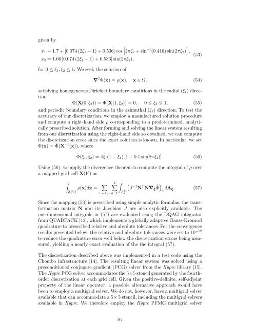
given byx 1 = 1.7 + [0.074 (2ξ 1 − 1) + 0.536] cos [ 2πξ 2 + sin −1 (0.416) sin(2πξ 2 ) ] ,x 2 = 1.66 [0.074 (2ξ 1 − 1) + 0.536] sin(2πξ 2 ),(53)for 0 ≤ ξ 1 , ξ 2 ≤ 1. We seek the solution of∇ 2 Φ(x) = ρ(x), x ∈ Ω, (54)satisfying homogeneous Dirichlet boundary conditions in the radial (ξ 1 ) directionΦ(X(0, ξ 2 )) = Φ(X(1, ξ 2 )) = 0, 0 ≤ ξ 2 ≤ 1, (55)and periodic boundary conditions in the azimuthal (ξ 2 ) direction. To test theaccuracy of our discretization, we employ a manufactured solution procedureand compute a right-hand side ρ corresponding to a predetermined, analyticallyprescribed solution. After forming and solving the linear system resultingfrom our discretization using the right-hand side so obtained, we can computethe discretization error since the exact solution is known. In particular, we setΦ(x) = ˜Φ(X −1 (x)), where˜Φ(ξ 1 , ξ 2 ) = 4ξ 1 (1 − ξ 1 ) [1 + 0.1 sin(8πξ 2 )] . (56)Using (56), we apply the divergence theorem to compute the integral of ρ overa mapped grid cell X(V ) as∫X(V )ρ(x)dx =∑ 2∑∫±=+,− d=1A ± d(J −1 N T N∇ ξ ˜Φ ) d dA ξ. (57)Since the mapping (53) is prescribed using simple analytic formulas, the transformationmatrix N and its Jacobian J are also explicitly available. Theone-dimensional integrals in (57) are evaluated using the DQAG integratorfrom QUADPACK [13], which implements a globally adaptive Gauss-Kronrodquadrature to prescribed relative and absolute tolerances. For the convergenceresults presented below, the relative and absolute tolerances were set to 10 −12to reduce the quadrature error well below the discretization errors being measured,yielding a nearly exact evaluation of the the integral (57).The discretization described above was implemented in a test code using theChombo infrastructure [14]. The resulting linear system was solved using apreconditioned conjugate gradient (PCG) solver from the Hypre library [15].The Hypre PCG solver accommodates the 5×5 stencil generated by the fourthorderdiscretization at each grid cell. Given the positive-definite, self-adjointproperty of the linear operator, a possible alternative approach would havebeen to employ a multigrid solver. We do not, however, have a multigrid solveravailable that can accommodate a 5×5 stencil, including the multigrid solversavailable in Hypre. We therefore employ the Hypre PFMG multigrid solver16
10 −2 N10 −310 −410 −510 −6Error10 −710 −810 −9L1 norm errorL2 norm errorMax norm errorN −410 −1010 −1110 1 10 2 10 3Fig. 5. Test problem convergence study.applied to a standard second-order discretization of (54) as a preconditionerfor CG. Beyond the issue of solver availability, it is generally acknowledgedthat the combination of a Krylov method with multigrid preconditioning yieldsa more robust solver, especially with variable coefficients.Figure 5 shows the L 1 , L 2 and max norm errors in the discrete solution of(54) using an N × N computational grid with N = 16, 32, 64, 128, 256 and512, plotted against N −4 . By L 1 and L 2 norms, we mean the discrete normscomputed using the solution error evaluated at cell centers, rather than continuousnorms computed using a reconstruction of the discrete solution overgrid cells. The fourth-order convergence rate is clearly observed. In each casethe PCG iteration was performed to a tolerance of 10 −10 on the relative L 2residual norm (the L 2 norm of the residual relative to that of the right handside). The multigrid preconditioner was solved to a relative tolerance of 10 −2in each iteration. Table 1 shows the relative residual at each iteration togetherwith an estimate of the local convergence rate for the finest grid N = 512. Apseudocolor plot of the N = 512 solution is shown on the right-hand side ofFigure 4.17
Page 1 and 2: High-Order, Finite-Volume Methods i
Page 3 and 4: the exact enforcement of the metric
Page 5: If we define control volumes in phy
Page 8 and 9: Alternative expressions to (17) are
Page 10: β 1 i+2 ed +e❞ ❞ ❞ d′❞β
Page 13 and 14: ✠Dirichlet boundaryDCBAFig. 3. Lo
Page 15: 10.80.60.40.20−0.2−0.4−0.6−
Page 21 and 22: 3Runge Kutta Stability Domain21Im z
Page 23 and 24: Magnitude of Amplification FactorRe
Page 26 and 27: L ∞ Error Norm for Base SchemeN c
Page 28 and 29: 10 0 Uniform Advection of Sinusoida
Page 30 and 31: Note that, in computational space,
Page 32 and 33: 10 0 Uniform Advection of Compact D
Page 34 and 35: and/or face-centered values. Among

High-Order, Finite-Volume Methods in Mapped Coordinates

You also want an ePaper? Increase the reach of your titles

Delete template?

Save as template?