High-Order, Finite-Volume Methods in Mapped Coordinates
High-Order, Finite-Volume Methods in Mapped Coordinates
High-Order, Finite-Volume Methods in Mapped Coordinates

You also want an ePaper? Increase the reach of your titles
YUMPU automatically turns print PDFs into web optimized ePapers that Google loves.
3Runge Kutta Stability Doma<strong>in</strong>21Im z0−1−2−3−2.5 −2 −1.5 −1 −0.5 0Re zFig. 6. Stability region of the classical Runge-Kutta scheme. The approximation bya semi-ellipse (77) is shown <strong>in</strong> blue.Thus,ū i ≡ h −D ∫V iu(x(ξ))dξ = ( [−1 ¯J) (uJ)i i− h212 ∇ ξu · ∇ ξ J + O ( h 4)] . (70)We require at least second-order approximations of the gradients and choosethe central differences⎡(∇ ξ u) d i= 1 ⎣ (uJ) i+e d2h ¯J i+e d− (uJ) i−e d¯J i−e d⎤⎦ + O ( h 2) (71)<strong>in</strong> each direction d. This choice is freestream preserv<strong>in</strong>g; the difference evaluatesto zero (with<strong>in</strong> roundoff) provided that the averages are <strong>in</strong>itialized suchthat, for constant u, uJ i ≡ u ¯J i .4.2 Time DiscretizationAs <strong>in</strong> [7], we discretize the semi-discrete system of ord<strong>in</strong>ary differential equations(61) us<strong>in</strong>g the explicit, four-stage, fourth-order classical Runge-Kuttascheme [17]. Consider the variable-coefficient problemdydt= A(x)y, (72)21